Clear sky#
This section reviews the clear sky modeling capabilities of pvlib-python.
pvlib-python supports two ways to generate clear sky irradiance:
A
Locationobject’sget_clearsky()method.The functions contained in the
clearskymodule, includingineichen()andsimplified_solis().
Users that work with simple time series data may prefer to use
get_clearsky(), while users
that want finer control, more explicit code, or work with
multidimensional data may prefer to use the basic functions in the
clearsky module.
The Location subsection demonstrates the easiest way to obtain a time series of clear sky data for a location. The Ineichen and Perez and Simplified Solis subsections detail the clear sky algorithms and input data. The Detect Clearsky subsection demonstrates the use of the clear sky detection algorithm.
We’ll need these imports for the examples below.
In [1]: import os

In [2]: import itertools

In [3]: import matplotlib.pyplot as plt

In [4]: import pandas as pd

In [5]: import pvlib

In [6]: from pvlib import clearsky, atmosphere, solarposition

In [7]: from pvlib.location import Location

In [8]: from pvlib.iotools import read_tmy3
Location#
The easiest way to obtain a time series of clear sky irradiance is to use a
Location object’s
get_clearsky() method. The
get_clearsky() method does the dirty
work of calculating solar position, extraterrestrial irradiance,
airmass, and atmospheric pressure, as appropriate, leaving the user to
only specify the most important parameters: time and atmospheric
attenuation. The time input must be a pandas.DatetimeIndex,
while the atmospheric attenuation inputs may be constants or arrays.
The get_clearsky() method always
returns a pandas.DataFrame.
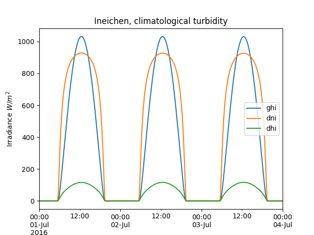
In [9]: tus = Location(32.2, -111, 'US/Arizona', 700, 'Tucson')

In [10]: times = pd.date_range(start='2016-07-01', end='2016-07-04', freq='1min', tz=tus.tz)

In [11]: cs = tus.get_clearsky(times)  # ineichen with climatology table by default

In [12]: cs.plot();

In [13]: plt.ylabel('Irradiance $W/m^2$');

In [14]: plt.title('Ineichen, climatological turbidity');
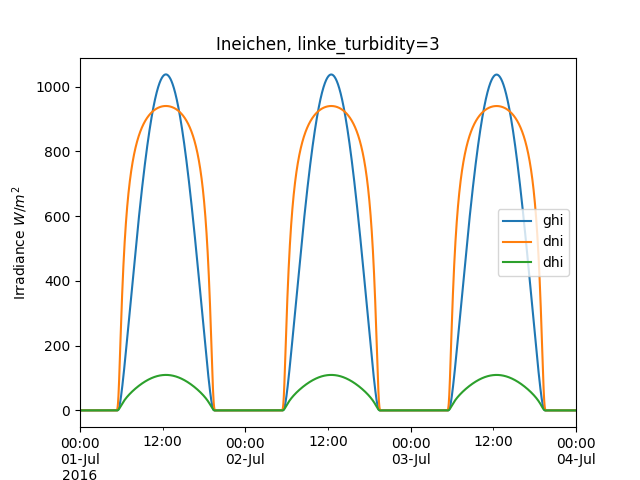
The get_clearsky() method accepts a
model keyword argument and propagates additional arguments to the
functions that do the computation.
In [15]: cs = tus.get_clearsky(times, model='ineichen', linke_turbidity=3)

In [16]: cs.plot();

In [17]: plt.title('Ineichen, linke_turbidity=3');

In [18]: plt.ylabel('Irradiance $W/m^2$');
In [19]: cs = tus.get_clearsky(times, model='simplified_solis', aod700=0.2, precipitable_water=3)

In [20]: cs.plot();

In [21]: plt.title('Simplfied Solis, aod700=0.2, precipitable_water=3');

In [22]: plt.ylabel('Irradiance $W/m^2$');
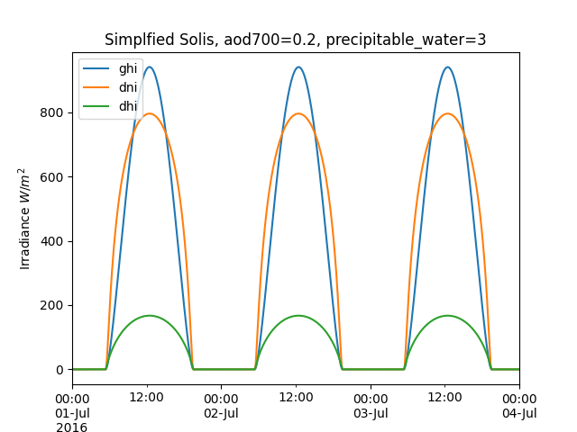
See the sections below for more detail on the clear sky models.
Ineichen and Perez#
The Ineichen and Perez clear sky model parameterizes irradiance in terms
of the Linke turbidity [Ine02]. pvlib-python implements this model in
the pvlib.clearsky.ineichen() function.
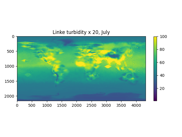
Turbidity data#
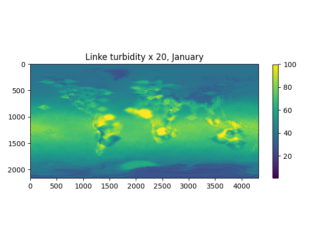
pvlib includes a file with monthly climatological turbidity values for the globe. The code below creates turbidity maps for a few months of the year. You could run it in a loop to create plots for all months.
In [23]: import calendar

In [24]: import os

In [25]: import h5py

In [26]: pvlib_path = os.path.dirname(os.path.abspath(pvlib.clearsky.__file__))

In [27]: filepath = os.path.join(pvlib_path, 'data', 'LinkeTurbidities.h5')

In [28]: def plot_turbidity_map(month, vmin=1, vmax=100):
   ....:     plt.figure();
   ....:     with h5py.File(filepath, 'r') as lt_h5_file:
   ....:         ltdata = lt_h5_file['LinkeTurbidity'][:, :, month-1]
   ....:     plt.imshow(ltdata, vmin=vmin, vmax=vmax);
   ....:     # data is in units of 20 x turbidity
   ....:     plt.title('Linke turbidity x 20, ' + calendar.month_name[month]);
   ....:     plt.colorbar(shrink=0.5);
   ....:     plt.tight_layout();
   ....:

In [29]: plot_turbidity_map(1)

In [30]: plot_turbidity_map(7)
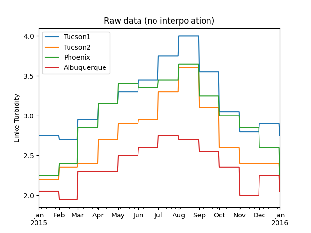
The lookup_linke_turbidity() function takes a
time, latitude, and longitude and gets the corresponding climatological
turbidity value for that time at those coordinates. By default, the
lookup_linke_turbidity() function will linearly
interpolate turbidity from month to month, assuming that the raw data is
valid on 15th of each month. This interpolation removes discontinuities
in multi-month PV models. Here’s a plot of a few locations in the
Southwest U.S. with and without interpolation. We chose points that are
relatively close so that you can get a better sense of the spatial noise
and variability of the data set. Note that the altitude of these sites
varies from 300 m to 1500 m.
In [31]: times = pd.date_range(start='2015-01-01', end='2016-01-01', freq='1D')
In [32]: sites = [(32, -111, 'Tucson1'), (32.2, -110.9, 'Tucson2'),
....: (33.5, -112.1, 'Phoenix'), (35.1, -106.6, 'Albuquerque')]
....:
In [33]: plt.figure();
In [34]: for lat, lon, name in sites:
....: turbidity = pvlib.clearsky.lookup_linke_turbidity(times, lat, lon, interp_turbidity=False)
....: turbidity.plot(label=name)
....:
In [35]: plt.legend();
In [36]: plt.title('Raw data (no interpolation)');
In [37]: plt.ylabel('Linke Turbidity');
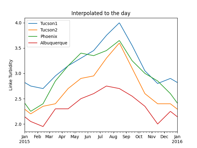
In [38]: plt.figure();
In [39]: for lat, lon, name in sites:
....: turbidity = pvlib.clearsky.lookup_linke_turbidity(times, lat, lon)
....: turbidity.plot(label=name)
....:
In [40]: plt.legend();
In [41]: plt.title('Interpolated to the day');
In [42]: plt.ylabel('Linke Turbidity');
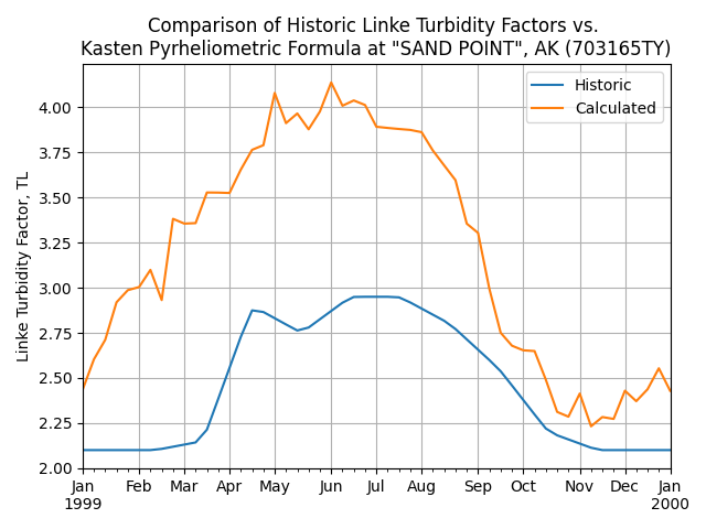
The kasten96_lt() function can be used to calculate
Linke turbidity [Kas96] as input to the clear sky Ineichen and Perez function.
The Kasten formulation requires precipitable water and broadband aerosol
optical depth (AOD). According to Molineaux, broadband AOD can be approximated
by a single measurement at 700-nm [Mol98]. An alternate broadband AOD
approximation from Bird and Hulstrom combines AOD measured at two
wavelengths [Bir80], and is implemented in
bird_hulstrom80_aod_bb().
In [43]: pvlib_data = os.path.join(os.path.dirname(pvlib.__file__), 'data')

In [44]: mbars = 100  # conversion factor from mbars to Pa

In [45]: tmy_file = os.path.join(pvlib_data, '703165TY.csv')  # TMY file

In [46]: tmy_data, tmy_header = read_tmy3(tmy_file, coerce_year=1999, map_variables=True)

In [47]: tl_historic = clearsky.lookup_linke_turbidity(time=tmy_data.index,
   ....:     latitude=tmy_header['latitude'], longitude=tmy_header['longitude'])
   ....:

In [48]: solpos = solarposition.get_solarposition(time=tmy_data.index,
   ....:     latitude=tmy_header['latitude'], longitude=tmy_header['longitude'],
   ....:     altitude=tmy_header['altitude'], pressure=tmy_data['pressure']*mbars,
   ....:     temperature=tmy_data['temp_air'])
   ....:

In [49]: am_rel = atmosphere.get_relative_airmass(solpos.apparent_zenith)

In [50]: am_abs = atmosphere.get_absolute_airmass(am_rel, tmy_data['pressure']*mbars)

In [51]: airmass = pd.concat([am_rel, am_abs], axis=1).rename(
   ....:     columns={0: 'airmass_relative', 1: 'airmass_absolute'})
   ....:

In [52]: tl_calculated = atmosphere.kasten96_lt(
   ....:     airmass.airmass_absolute, tmy_data['precipitable_water'],
   ....:     tmy_data['AOD (unitless)'])
   ....:

In [53]: tl = pd.concat([tl_historic, tl_calculated], axis=1).rename(
   ....:     columns={0:'Historic', 1:'Calculated'})
   ....:

In [54]: tl.index = tmy_data.index.tz_convert(None)  # remove timezone

In [55]: tl.resample('W').mean().plot();

In [56]: plt.grid()

In [57]: plt.title('Comparison of Historic Linke Turbidity Factors vs. \n'
   ....:     'Kasten Pyrheliometric Formula at {name:s}, {state:s} ({usaf:d}TY)'.format(
   ....:     name=tmy_header['Name'], state=tmy_header['State'], usaf=tmy_header['USAF']));
   ....:

In [58]: plt.ylabel('Linke Turbidity Factor, TL');

In [59]: plt.tight_layout()
Examples#
A clear sky time series using only basic pvlib functions.
In [60]: latitude, longitude, tz, altitude, name = 32.2, -111, 'US/Arizona', 700, 'Tucson'

In [61]: times = pd.date_range(start='2014-01-01', end='2014-01-02', freq='1Min', tz=tz)

In [62]: solpos = pvlib.solarposition.get_solarposition(times, latitude, longitude)

In [63]: apparent_zenith = solpos['apparent_zenith']

In [64]: airmass = pvlib.atmosphere.get_relative_airmass(apparent_zenith)

In [65]: pressure = pvlib.atmosphere.alt2pres(altitude)

In [66]: airmass = pvlib.atmosphere.get_absolute_airmass(airmass, pressure)

In [67]: linke_turbidity = pvlib.clearsky.lookup_linke_turbidity(times, latitude, longitude)

In [68]: dni_extra = pvlib.irradiance.get_extra_radiation(times)

# an input is a pandas Series, so solis is a DataFrame
In [69]: ineichen = clearsky.ineichen(apparent_zenith, airmass, linke_turbidity, altitude, dni_extra)

In [70]: plt.figure();

In [71]: ax = ineichen.plot()

In [72]: ax.set_ylabel('Irradiance $W/m^2$');

In [73]: ax.set_title('Ineichen Clear Sky Model');

In [74]: ax.legend(loc=2);
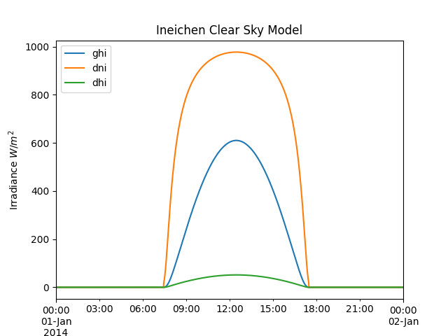
The input data types determine the returned output type. Array input results in an OrderedDict of array output, and Series input results in a DataFrame output. The keys are ‘ghi’, ‘dni’, and ‘dhi’.
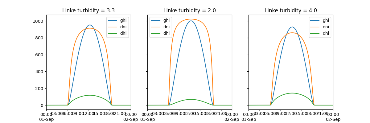
Grid with a clear sky irradiance for a few turbidity values.
In [75]: times = pd.date_range(start='2014-09-01', end='2014-09-02', freq='1Min', tz=tz)

In [76]: solpos = pvlib.solarposition.get_solarposition(times, latitude, longitude)

In [77]: apparent_zenith = solpos['apparent_zenith']

In [78]: airmass = pvlib.atmosphere.get_relative_airmass(apparent_zenith)

In [79]: pressure = pvlib.atmosphere.alt2pres(altitude)

In [80]: airmass = pvlib.atmosphere.get_absolute_airmass(airmass, pressure)

In [81]: linke_turbidity = pvlib.clearsky.lookup_linke_turbidity(times, latitude, longitude)

In [82]: print('climatological linke_turbidity = {}'.format(linke_turbidity.mean()))
climatological linke_turbidity = 3.329496820286459

In [83]: dni_extra = pvlib.irradiance.get_extra_radiation(times)

In [84]: linke_turbidities = [linke_turbidity.mean(), 2, 4]

In [85]: fig, axes = plt.subplots(ncols=3, nrows=1, sharex=True, sharey=True, squeeze=True, figsize=(12, 4))

In [86]: axes = axes.flatten()

In [87]: for linke_turbidity, ax in zip(linke_turbidities, axes):
   ....:     ineichen = clearsky.ineichen(apparent_zenith, airmass, linke_turbidity, altitude, dni_extra)
   ....:     ineichen.plot(ax=ax, title='Linke turbidity = {:0.1f}'.format(linke_turbidity));
   ....:

In [88]: ax.legend(loc=1);
Simplified Solis#
The Simplified Solis model parameterizes irradiance in terms of
precipitable water and aerosol optical depth [Ine08ss]. pvlib-python
implements this model in the pvlib.clearsky.simplified_solis()
function.
Aerosol and precipitable water data#
There are a number of sources for aerosol and precipitable water data
of varying accuracy, global coverage, and temporal resolution.
Ground based aerosol data can be obtained from
Aeronet. Precipitable water can be
derived from surface relative humidity using functions such as
pvlib.atmosphere.gueymard94_pw().
Numerous gridded products from satellites, weather models, and climate models
contain one or both of aerosols and precipitable water. Consider data
from the ECMWF ERA5,
NASA MERRA-2,
and SoDa.
Aerosol optical depth (AOD) is a function of wavelength, and the Simplified
Solis model requires AOD at 700 nm.
angstrom_aod_at_lambda() is useful for converting
AOD between different wavelengths using the Angstrom turbidity model. The
Angstrom exponent, \(\alpha\), can be calculated from AOD at two
wavelengths with angstrom_alpha().
[Ine08con], [Ine16], [Ang61].
In [89]: aod1240nm = 1.2  # fictitious AOD measured at 1240-nm

In [90]: aod550nm = 3.1  # fictitious AOD measured at 550-nm

In [91]: alpha_exponent = atmosphere.angstrom_alpha(aod1240nm, 1240, aod550nm, 550)

In [92]: aod700nm = atmosphere.angstrom_aod_at_lambda(aod1240nm, 1240, alpha_exponent, 700)

In [93]: aod380nm = atmosphere.angstrom_aod_at_lambda(aod550nm, 550, alpha_exponent, 380)

In [94]: aod500nm = atmosphere.angstrom_aod_at_lambda(aod550nm, 550, alpha_exponent, 500)

In [95]: aod_bb = atmosphere.bird_hulstrom80_aod_bb(aod380nm, aod500nm)

In [96]: print('compare AOD at 700-nm = {:g}, to estimated broadband AOD = {:g}, '
   ....:     'with alpha = {:g}'.format(aod700nm, aod_bb, alpha_exponent))
   ....:
compare AOD at 700-nm = 2.33931, to estimated broadband AOD = 2.52936, with alpha = 1.16745
Examples#
A clear sky time series using only basic pvlib functions.
In [97]: latitude, longitude, tz, altitude, name = 32.2, -111, 'US/Arizona', 700, 'Tucson'

In [98]: times = pd.date_range(start='2014-01-01', end='2014-01-02', freq='1Min', tz=tz)

In [99]: solpos = pvlib.solarposition.get_solarposition(times, latitude, longitude)

In [100]: apparent_elevation = solpos['apparent_elevation']

In [101]: aod700 = 0.1

In [102]: precipitable_water = 1

In [103]: pressure = pvlib.atmosphere.alt2pres(altitude)

In [104]: dni_extra = pvlib.irradiance.get_extra_radiation(times)

# an input is a Series, so solis is a DataFrame
In [105]: solis = clearsky.simplified_solis(apparent_elevation, aod700, precipitable_water,
   .....:                                   pressure, dni_extra)
   .....:

In [106]: ax = solis.plot();

In [107]: ax.set_ylabel('Irradiance $W/m^2$');

In [108]: ax.set_title('Simplified Solis Clear Sky Model');

In [109]: ax.legend(loc=2);
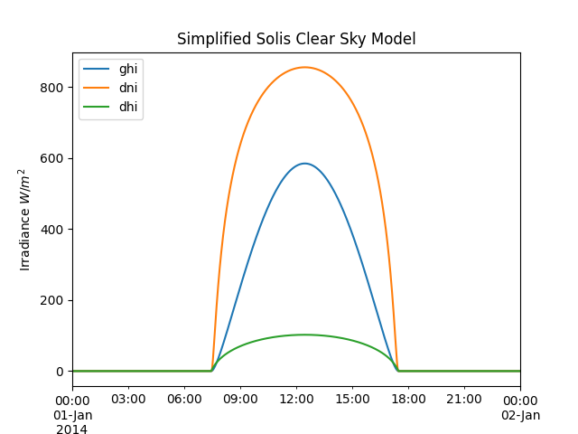
The input data types determine the returned output type. Array input results in an OrderedDict of array output, and Series input results in a DataFrame output. The keys are ‘ghi’, ‘dni’, and ‘dhi’.
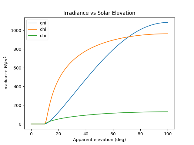
Irradiance as a function of solar elevation.
In [110]: apparent_elevation = pd.Series(np.linspace(-10, 90, 101))

In [111]: aod700 = 0.1

In [112]: precipitable_water = 1

In [113]: pressure = 101325

In [114]: dni_extra = 1364

In [115]: solis = clearsky.simplified_solis(apparent_elevation, aod700,
   .....:                                   precipitable_water, pressure, dni_extra)
   .....:

In [116]: ax = solis.plot();

In [117]: ax.set_xlabel('Apparent elevation (deg)');

In [118]: ax.set_ylabel('Irradiance $W/m^2$');

In [119]: ax.set_title('Irradiance vs Solar Elevation')
Out[119]: Text(0.5, 1.0, 'Irradiance vs Solar Elevation')

In [120]: ax.legend(loc=2);
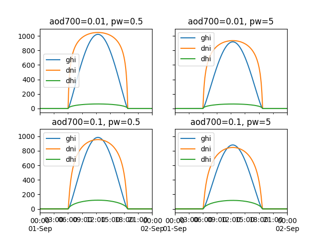
Grid with clear sky irradiance for a few PW and AOD values.
In [121]: times = pd.date_range(start='2014-09-01', end='2014-09-02', freq='1Min', tz=tz)

In [122]: solpos = pvlib.solarposition.get_solarposition(times, latitude, longitude)

In [123]: apparent_elevation = solpos['apparent_elevation']

In [124]: pressure = pvlib.atmosphere.alt2pres(altitude)

In [125]: dni_extra = pvlib.irradiance.get_extra_radiation(times)

In [126]: aod700 = [0.01, 0.1]

In [127]: precipitable_water = [0.5, 5]

In [128]: fig, axes = plt.subplots(ncols=2, nrows=2, sharex=True, sharey=True, squeeze=True)

In [129]: axes = axes.flatten()

In [130]: for (aod, pw), ax in zip(itertools.chain(itertools.product(aod700, precipitable_water)), axes):
   .....:     cs = clearsky.simplified_solis(apparent_elevation, aod, pw, pressure, dni_extra)
   .....:     cs.plot(ax=ax, title='aod700={}, pw={}'.format(aod, pw))
   .....:
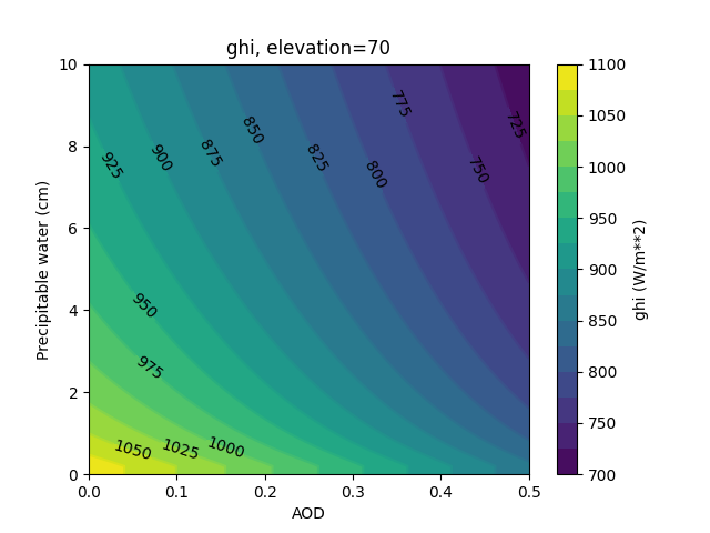
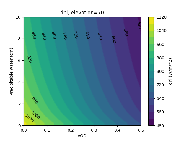
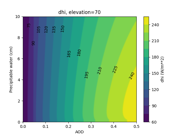
Contour plots of irradiance as a function of both PW and AOD.
In [131]: aod700 = np.linspace(0, 0.5, 101)

In [132]: precipitable_water = np.linspace(0, 10, 101)

In [133]: apparent_elevation = 70

In [134]: pressure = 101325

In [135]: dni_extra = 1364

In [136]: aod700, precipitable_water = np.meshgrid(aod700, precipitable_water)

# inputs are arrays, so solis is an OrderedDict
In [137]: solis = clearsky.simplified_solis(apparent_elevation, aod700,
   .....:                                   precipitable_water, pressure,
   .....:                                   dni_extra)
   .....:

In [138]: n = 15

In [139]: vmin = None

In [140]: vmax = None

In [141]: def plot_solis(key):
   .....:     irrad = solis[key]
   .....:     fig, ax = plt.subplots()
   .....:     im = ax.contour(aod700, precipitable_water, irrad[:, :], n, vmin=vmin, vmax=vmax)
   .....:     imf = ax.contourf(aod700, precipitable_water, irrad[:, :], n, vmin=vmin, vmax=vmax)
   .....:     ax.set_xlabel('AOD')
   .....:     ax.set_ylabel('Precipitable water (cm)')
   .....:     ax.clabel(im, colors='k', fmt='%.0f')
   .....:     fig.colorbar(imf, label='{} (W/m**2)'.format(key))
   .....:     ax.set_title('{}, elevation={}'.format(key, apparent_elevation))
   .....:
In [142]: plot_solis('ghi')


In [143]: plot_solis('dni')


In [144]: plot_solis('dhi')
Detect Clearsky#
The detect_clearsky() function implements the
[Ren16] algorithm to detect the clear and cloudy points of a time
series. The algorithm was designed and validated for analyzing GHI time
series only. Users may attempt to apply it to other types of time series
data using different filter settings, but should be skeptical of the
results.
The algorithm detects clear sky times by comparing statistics for a measured time series and an expected clearsky time series. Statistics are calculated using a sliding time window (e.g., 10 minutes). An iterative algorithm identifies clear periods, uses the identified periods to estimate bias in the clearsky data, scales the clearsky data and repeats.
Clear times are identified by meeting 5 criteria. Default values for these thresholds are appropriate for 10 minute windows of 1 minute GHI data.
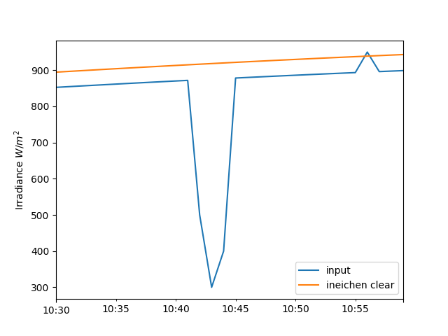
Next, we show a simple example of applying the algorithm to synthetic GHI data. We first generate and plot the clear sky and measured data.
In [145]: abq = Location(35.04, -106.62, altitude=1619)

In [146]: times = pd.date_range(start='2012-04-01 10:30:00', tz='Etc/GMT+7', periods=30, freq='1min')

In [147]: cs = abq.get_clearsky(times)

# scale clear sky data to account for possibility of different turbidity
In [148]: ghi = cs['ghi']*.953

# add a cloud event
In [149]: ghi['2012-04-01 10:42:00':'2012-04-01 10:44:00'] = [500, 300, 400]

# add an overirradiance event
In [150]: ghi['2012-04-01 10:56:00'] = 950

In [151]: fig, ax = plt.subplots()

In [152]: ghi.plot(label='input');

In [153]: cs['ghi'].plot(label='ineichen clear');

In [154]: ax.set_ylabel('Irradiance $W/m^2$');

In [155]: plt.legend(loc=4);
Now we run the synthetic data and clear sky estimate through the
detect_clearsky() function.
In [156]: clear_samples = clearsky.detect_clearsky(ghi, cs['ghi'])

In [157]: fig, ax = plt.subplots()

In [158]: clear_samples.astype(int).plot();

In [159]: ax.set_ylabel('Clear (1) or Cloudy (0)');
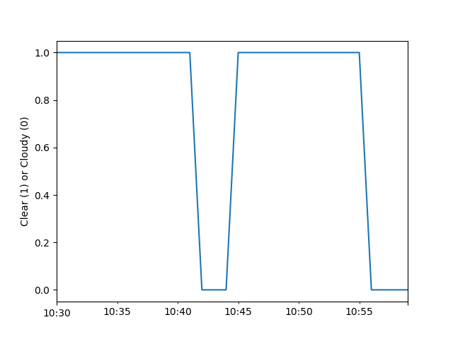
The algorithm detected the cloud event and the overirradiance event.
References#
- Ine02(1,2)
P. Ineichen and R. Perez, “A New airmass independent formulation for the Linke turbidity coefficient”, Solar Energy, 73, pp. 151-157, 2002.
- Ine08ss
P. Ineichen, “A broadband simplified version of the Solis clear sky model,” Solar Energy, 82, 758-762 (2008).
- Ine16(1,2)
P. Ineichen, “Validation of models that estimate the clear sky global and beam solar irradiance,” Solar Energy, 132, 332-344 (2016).
- Ine08con
P. Ineichen, “Conversion function between the Linke turbidity and the atmospheric water vapor and aerosol content”, Solar Energy, 82, 1095 (2008).
- Ren12
M. Reno, C. Hansen, and J. Stein, “Global Horizontal Irradiance Clear Sky Models: Implementation and Analysis”, Sandia National Laboratories, SAND2012-2389, 2012.
- Ren16
Reno, M.J. and C.W. Hansen, “Identification of periods of clear sky irradiance in time series of GHI measurements” Renewable Energy, v90, p. 520-531, 2016.
- Mol98
B. Molineaux, P. Ineichen, and N. O’Neill, “Equivalence of pyrheliometric and monochromatic aerosol optical depths at a single key wavelength.,” Appl. Opt., vol. 37, no. 30, pp. 7008–18, Oct. 1998.
- Kas96
F. Kasten, “The linke turbidity factor based on improved values of the integral Rayleigh optical thickness,” Sol. Energy, vol. 56, no. 3, pp. 239–244, Mar. 1996.
- Bir80
R. E. Bird and R. L. Hulstrom, “Direct Insolation Models,” 1980.
- Ang61
A. ÅNGSTRÖM, “Techniques of Determinig the Turbidity of the Atmosphere,” Tellus A, vol. 13, no. 2, pp. 214–223, 1961.