Intro Tutorial#
This page contains introductory examples of pvlib python usage.
Modeling paradigms#
The backbone of pvlib-python is well-tested procedural code that implements PV system models. pvlib-python also provides a collection of classes for users that prefer object-oriented programming. These classes can help users keep track of data in a more organized way, provide some “smart” functions with more flexible inputs, and simplify the modeling process for common situations. The classes do not add any algorithms beyond what’s available in the procedural code, and most of the object methods are simple wrappers around the corresponding procedural code.
Let’s use each of these pvlib modeling paradigms to calculate the yearly energy yield for a given hardware configuration at a handful of sites listed below.
In [1]: import pvlib

In [2]: import pandas as pd

In [3]: import matplotlib.pyplot as plt

# latitude, longitude, name, altitude, timezone
In [4]: coordinates = [
   ...:     (32.2, -111.0, 'Tucson', 700, 'Etc/GMT+7'),
   ...:     (35.1, -106.6, 'Albuquerque', 1500, 'Etc/GMT+7'),
   ...:     (37.8, -122.4, 'San Francisco', 10, 'Etc/GMT+8'),
   ...:     (52.5, 13.4, 'Berlin', 34, 'Etc/GMT-1'),
   ...: ]
   ...:

# get the module and inverter specifications from SAM
In [5]: sandia_modules = pvlib.pvsystem.retrieve_sam('SandiaMod')

In [6]: sapm_inverters = pvlib.pvsystem.retrieve_sam('cecinverter')

In [7]: module = sandia_modules['Canadian_Solar_CS5P_220M___2009_']

In [8]: inverter = sapm_inverters['ABB__MICRO_0_25_I_OUTD_US_208__208V_']

In [9]: temperature_model_parameters = pvlib.temperature.TEMPERATURE_MODEL_PARAMETERS['sapm']['open_rack_glass_glass']
In order to retrieve meteorological data for the simulation, we can make use of the IO Tools module. In this example we will be using PVGIS, one of the data sources available, to retrieve a Typical Meteorological Year (TMY) which includes irradiation, temperature and wind speed.
In [10]: tmys = []

In [11]: for location in coordinates:
   ....:     latitude, longitude, name, altitude, timezone = location
   ....:     weather = pvlib.iotools.get_pvgis_tmy(latitude, longitude)[0]
   ....:     weather.index.name = "utc_time"
   ....:     tmys.append(weather)
   ....:
Procedural#
The straightforward procedural code can be used for all modeling steps in pvlib-python.
The following code demonstrates how to use the procedural code to accomplish our system modeling goal:
In [12]: system = {'module': module, 'inverter': inverter,
....: 'surface_azimuth': 180}
....:
In [13]: energies = {}
In [14]: for location, weather in zip(coordinates, tmys):
....: latitude, longitude, name, altitude, timezone = location
....: system['surface_tilt'] = latitude
....: solpos = pvlib.solarposition.get_solarposition(
....: time=weather.index,
....: latitude=latitude,
....: longitude=longitude,
....: altitude=altitude,
....: temperature=weather["temp_air"],
....: pressure=pvlib.atmosphere.alt2pres(altitude),
....: )
....: dni_extra = pvlib.irradiance.get_extra_radiation(weather.index)
....: airmass = pvlib.atmosphere.get_relative_airmass(solpos['apparent_zenith'])
....: pressure = pvlib.atmosphere.alt2pres(altitude)
....: am_abs = pvlib.atmosphere.get_absolute_airmass(airmass, pressure)
....: aoi = pvlib.irradiance.aoi(
....: system['surface_tilt'],
....: system['surface_azimuth'],
....: solpos["apparent_zenith"],
....: solpos["azimuth"],
....: )
....: total_irradiance = pvlib.irradiance.get_total_irradiance(
....: system['surface_tilt'],
....: system['surface_azimuth'],
....: solpos['apparent_zenith'],
....: solpos['azimuth'],
....: weather['dni'],
....: weather['ghi'],
....: weather['dhi'],
....: dni_extra=dni_extra,
....: model='haydavies',
....: )
....: cell_temperature = pvlib.temperature.sapm_cell(
....: total_irradiance['poa_global'],
....: weather["temp_air"],
....: weather["wind_speed"],
....: **temperature_model_parameters,
....: )
....: effective_irradiance = pvlib.pvsystem.sapm_effective_irradiance(
....: total_irradiance['poa_direct'],
....: total_irradiance['poa_diffuse'],
....: am_abs,
....: aoi,
....: module,
....: )
....: dc = pvlib.pvsystem.sapm(effective_irradiance, cell_temperature, module)
....: ac = pvlib.inverter.sandia(dc['v_mp'], dc['p_mp'], inverter)
....: annual_energy = ac.sum()
....: energies[name] = annual_energy
....:
In [15]: energies = pd.Series(energies)
# based on the parameters specified above, these are in W*hrs
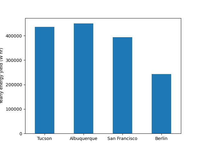
In [16]: print(energies)
Tucson 435946.033478
Albuquerque 449905.612212
San Francisco 393749.369318
Berlin 243230.830516
dtype: float64
In [17]: energies.plot(kind='bar', rot=0)
Out[17]: <AxesSubplot:>
In [18]: plt.ylabel('Yearly energy yield (W hr)')
Out[18]: Text(0, 0.5, 'Yearly energy yield (W hr)')
Object oriented (Location, Mount, Array, PVSystem, ModelChain)#
The object oriented paradigm uses a model with three main concepts:
System design (modules, inverters etc.) is represented by
PVSystem,Array, andFixedMount/SingleAxisTrackerMountobjects.A particular place on the planet is represented by a
Locationobject.The modeling chain used to calculate power output for a particular system and location is represented by a
ModelChainobject.
This can be a useful paradigm if you prefer to think about the PV system and its location as separate concepts or if you develop your own ModelChain subclasses. It can also be helpful if you make extensive use of Location-specific methods for other calculations.
The following code demonstrates how to use
Location,
PVSystem, and
ModelChain objects to accomplish our
system modeling goal. ModelChain objects provide convenience methods
that can provide default selections for models and can also fill
necessary input with modeled data. For example, no air temperature
or wind speed data is provided in the input weather DataFrame,
so the ModelChain object defaults to 20 C and 0 m/s. Also, no irradiance
transposition model is specified (keyword argument transposition_model for
ModelChain) so the ModelChain defaults to the haydavies model. In this
example, ModelChain infers the DC power model from the module provided
by examining the parameters defined for the module.
In [19]: from pvlib.pvsystem import PVSystem, Array, FixedMount

In [20]: from pvlib.location import Location

In [21]: from pvlib.modelchain import ModelChain

In [22]: energies = {}

In [23]: for location, weather in zip(coordinates, tmys):
   ....:     latitude, longitude, name, altitude, timezone = location
   ....:     location = Location(
   ....:         latitude,
   ....:         longitude,
   ....:         name=name,
   ....:         altitude=altitude,
   ....:         tz=timezone,
   ....:     )
   ....:     mount = FixedMount(surface_tilt=latitude, surface_azimuth=180)
   ....:     array = Array(
   ....:         mount=mount,
   ....:         module_parameters=module,
   ....:         temperature_model_parameters=temperature_model_parameters,
   ....:     )
   ....:     system = PVSystem(arrays=[array], inverter_parameters=inverter)
   ....:     mc = ModelChain(system, location)
   ....:     mc.run_model(weather)
   ....:     annual_energy = mc.results.ac.sum()
   ....:     energies[name] = annual_energy
   ....:

In [24]: energies = pd.Series(energies)

# based on the parameters specified above, these are in W*hrs
In [25]: print(energies)
Tucson           435945.540454
Albuquerque      449905.103839
San Francisco    393749.728807
Berlin           243230.970659
dtype: float64

In [26]: energies.plot(kind='bar', rot=0)
Out[26]: <AxesSubplot:>

In [27]: plt.ylabel('Yearly energy yield (W hr)')
Out[27]: Text(0, 0.5, 'Yearly energy yield (W hr)')
