Forecasting
pvlib-python provides a set of functions and classes that make it easy to obtain weather forecast data and convert that data into a PV power forecast. Users can retrieve standardized weather forecast data relevant to PV power modeling from NOAA/NCEP/NWS models including the GFS, NAM, RAP, HRRR, and the NDFD. A PV power forecast can then be obtained using the weather data as inputs to the comprehensive modeling capabilities of PVLIB-Python. Standardized, open source, reference implementations of forecast methods using publicly available data may help advance the state-of-the-art of solar power forecasting.
pvlib-python uses Unidata’s Siphon library to simplify access to real-time forecast data hosted on the Unidata THREDDS catalog. Siphon is great for programatic access of THREDDS data, but we also recommend using tools such as Panoply to easily browse the catalog and become more familiar with its contents.
We do not know of a similarly easy way to access archives of forecast data.
This document demonstrates how to use pvlib-python to create a PV power forecast using these tools. The forecast and forecast_to_power Jupyter notebooks provide additional example code.
Warning
The forecast module algorithms and features are highly experimental. The API may change, the functionality may be consolidated into an io module, or the module may be separated into its own package.
Note
This documentation is difficult to reliably build on readthedocs. If you do not see images, try building the documentation on your own machine or see the notebooks linked to above.
Accessing Forecast Data
The Siphon library provides access to, among others, forecasts from the
Global Forecast System (GFS), North American Model (NAM), High
Resolution Rapid Refresh (HRRR), Rapid Refresh (RAP), and National
Digital Forecast Database (NDFD) on a Unidata THREDDS server.
Unfortunately, many of these models use different names to describe the
same quantity (or a very similar one), and not all variables are present
in all models. For example, on the THREDDS server, the GFS has a field
named
Total_cloud_cover_entire_atmosphere_Mixed_intervals_Average,
while the NAM has a field named
Total_cloud_cover_entire_atmosphere_single_layer, and a
similar field in the HRRR is named
Total_cloud_cover_entire_atmosphere.
PVLIB-Python aims to simplify the access of the model fields relevant
for solar power forecasts. Model data accessed with PVLIB-Python is
returned as a pandas DataFrame with consistent column names:
temp_air, wind_speed, total_clouds, low_clouds, mid_clouds,
high_clouds, dni, dhi, ghi
. To accomplish this, we use an
object-oriented framework in which each weather model is represented by
a class that inherits from a parent
ForecastModel class.
The parent ForecastModel class contains the
common code for accessing and parsing the data using Siphon, while the
child model-specific classes (GFS,
HRRR, etc.) contain the code necessary to
map and process that specific model’s data to the standardized fields.
The code below demonstrates how simple it is to access and plot forecast data using PVLIB-Python. First, we set up make the basic imports and then set the location and time range data.
In [1]: import pandas as pd

In [2]: import matplotlib.pyplot as plt

In [3]: import datetime

# import pvlib forecast models
In [4]: from pvlib.forecast import GFS, NAM, NDFD, HRRR, RAP

# specify location (Tucson, AZ)
In [5]: latitude, longitude, tz = 32.2, -110.9, 'US/Arizona'

# specify time range.
In [6]: start = pd.Timestamp(datetime.date.today(), tz=tz)

In [7]: end = start + pd.Timedelta(days=7)

In [8]: irrad_vars = ['ghi', 'dni', 'dhi']
Next, we instantiate a GFS model object and get the forecast data from Unidata.
# GFS model, defaults to 0.5 degree resolution
# 0.25 deg available
In [9]: model = GFS()

# retrieve data. returns pandas.DataFrame object
In [10]: raw_data = model.get_data(latitude, longitude, start, end)

In [11]: print(raw_data.head())
                           Downward_Short-Wave_Radiation_Flux_surface_Mixed_intervals_Average              ...               v-component_of_wind_isobaric
2018-09-17 09:00:00-07:00                                                0.0                               ...                                  -1.933579
2018-09-17 12:00:00-07:00                                                0.0                               ...                                  -1.158044
2018-09-17 15:00:00-07:00                                               90.0                               ...                                  -0.640168
2018-09-17 18:00:00-07:00                                              359.0                               ...                                  -2.382595
2018-09-17 21:00:00-07:00                                              870.0                               ...                                  -3.292986

[5 rows x 11 columns]
It will be useful to process this data before using it with pvlib. For example, the column names are non-standard, the temperature is in Kelvin, the wind speed is broken into east/west and north/south components, and most importantly, most of the irradiance data is missing. The forecast module provides a number of methods to fix these problems.
In [12]: data = raw_data

# rename the columns according the key/value pairs in model.variables.
In [13]: data = model.rename(data)

# convert temperature
In [14]: data['temp_air'] = model.kelvin_to_celsius(data['temp_air'])

# convert wind components to wind speed
In [15]: data['wind_speed'] = model.uv_to_speed(data)

# calculate irradiance estimates from cloud cover.
# uses a cloud_cover to ghi to dni model or a
# uses a cloud cover to transmittance to irradiance model.
# this step is discussed in more detail in the next section
In [16]: irrad_data = model.cloud_cover_to_irradiance(data['total_clouds'])

In [17]: data = data.join(irrad_data, how='outer')

# keep only the final data
In [18]: data = data[model.output_variables]

In [19]: print(data.head())
                            temp_air     ...       high_clouds
2018-09-17 09:00:00-07:00  25.411072     ...               2.0
2018-09-17 12:00:00-07:00  23.252838     ...               1.0
2018-09-17 15:00:00-07:00  32.772034     ...               0.0
2018-09-17 18:00:00-07:00  49.186951     ...               0.0
2018-09-17 21:00:00-07:00  51.744659     ...               0.0

[5 rows x 9 columns]
Much better.
The GFS class’s
process_data() method combines these steps
in a single function. In fact, each forecast model class
implements its own process_data method since the data from each
weather model is slightly different. The process_data functions are
designed to be explicit about how the data is being processed, and users
are strongly encouraged to read the source code of these methods.
In [20]: data = model.process_data(raw_data)

In [21]: print(data.head())
                            temp_air     ...       high_clouds
2018-09-17 09:00:00-07:00  25.411072     ...               2.0
2018-09-17 12:00:00-07:00  23.252838     ...               1.0
2018-09-17 15:00:00-07:00  32.772034     ...               0.0
2018-09-17 18:00:00-07:00  49.186951     ...               0.0
2018-09-17 21:00:00-07:00  51.744659     ...               0.0

[5 rows x 9 columns]
Users can easily implement their own process_data methods on
inherited classes or implement similar stand-alone functions.
The forecast model classes also implement a
get_processed_data() method that
combines the get_data() and
process_data() calls.
In [22]: data = model.get_processed_data(latitude, longitude, start, end)

In [23]: print(data.head())
                            temp_air     ...       high_clouds
2018-09-17 09:00:00-07:00  25.411072     ...               2.0
2018-09-17 12:00:00-07:00  23.252838     ...               1.0
2018-09-17 15:00:00-07:00  32.772034     ...               0.0
2018-09-17 18:00:00-07:00  49.186951     ...               0.0
2018-09-17 21:00:00-07:00  51.744659     ...               0.0

[5 rows x 9 columns]
Cloud cover and radiation
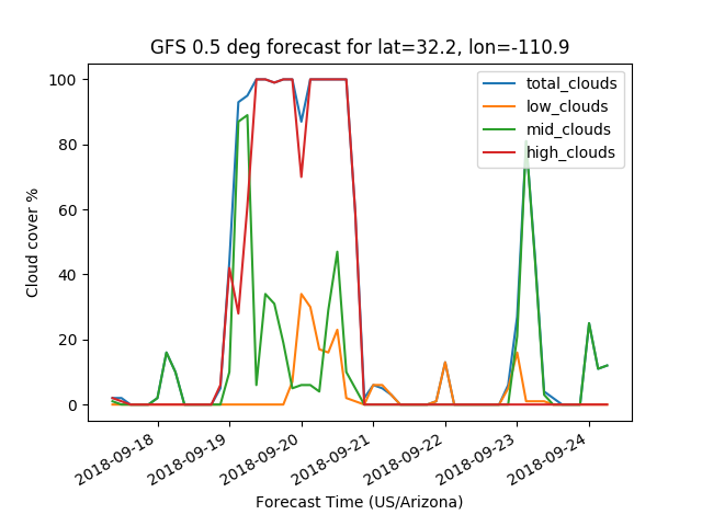
All of the weather models currently accessible by pvlib include one or more cloud cover forecasts. For example, below we plot the GFS cloud cover forecasts.
# plot cloud cover percentages
In [24]: cloud_vars = ['total_clouds', 'low_clouds',
   ....:               'mid_clouds', 'high_clouds']
   ....:

In [25]: data[cloud_vars].plot();

In [26]: plt.ylabel('Cloud cover %');

In [27]: plt.xlabel('Forecast Time ({})'.format(tz));

In [28]: plt.title('GFS 0.5 deg forecast for lat={}, lon={}'
   ....:           .format(latitude, longitude));
   ....:

In [29]: plt.legend();
However, many of forecast models do not include radiation components in their output fields, or if they do then the radiation fields suffer from poor solar position or radiative transfer algorithms. It is often more accurate to create empirically derived radiation forecasts from the weather models’ cloud cover forecasts.
PVLIB-Python provides two basic ways to convert cloud cover forecasts to irradiance forecasts. One method assumes a linear relationship between cloud cover and GHI, applies the scaling to a clear sky climatology, and then uses the DISC model to calculate DNI. The second method assumes a linear relationship between cloud cover and atmospheric transmittance, and then uses the Liu-Jordan [Liu60] model to calculate GHI, DNI, and DHI.
Caveat emptor: these algorithms are not rigorously verified! The purpose of the forecast module is to provide a few exceedingly simple options for users to play with before they develop their own models. We strongly encourage pvlib users first read the source code and second to implement new cloud cover to irradiance algorithms.
The essential parts of the clear sky scaling algorithm are as follows. Clear sky scaling of climatological GHI is also used in Larson et. al. [Lar16].
solpos = location.get_solarposition(cloud_cover.index)
cs = location.get_clearsky(cloud_cover.index, model='ineichen')
# offset and cloud cover in decimal units here
# larson et. al. use offset = 0.35
ghi = (offset + (1 - offset) * (1 - cloud_cover)) * ghi_clear
dni = disc(ghi, solpos['zenith'], cloud_cover.index)['dni']
dhi = ghi - dni * np.cos(np.radians(solpos['zenith']))
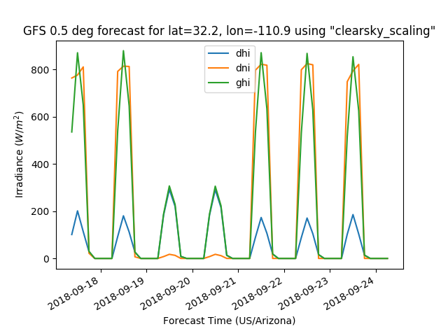
The figure below shows the result of the total cloud cover to irradiance conversion using the clear sky scaling algorithm.
# plot irradiance data
In [30]: data = model.rename(raw_data)

In [31]: irrads = model.cloud_cover_to_irradiance(data['total_clouds'], how='clearsky_scaling')

In [32]: irrads.plot();

In [33]: plt.ylabel('Irradiance ($W/m^2$)');

In [34]: plt.xlabel('Forecast Time ({})'.format(tz));

In [35]: plt.title('GFS 0.5 deg forecast for lat={}, lon={} using "clearsky_scaling"'
   ....:           .format(latitude, longitude));
   ....:

In [36]: plt.legend();
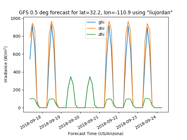
The essential parts of the Liu-Jordan cloud cover to irradiance algorithm are as follows.
# cloud cover in percentage units here
transmittance = ((100.0 - cloud_cover) / 100.0) * 0.75
# irrads is a DataFrame containing ghi, dni, dhi
irrads = liujordan(apparent_zenith, transmittance, airmass_absolute)
The figure below shows the result of the Liu-Jordan total cloud cover to irradiance conversion.
# plot irradiance data
In [37]: irrads = model.cloud_cover_to_irradiance(data['total_clouds'], how='liujordan')

In [38]: irrads.plot();

In [39]: plt.ylabel('Irradiance ($W/m^2$)');

In [40]: plt.xlabel('Forecast Time ({})'.format(tz));

In [41]: plt.title('GFS 0.5 deg forecast for lat={}, lon={} using "liujordan"'
   ....:           .format(latitude, longitude));
   ....:

In [42]: plt.legend();
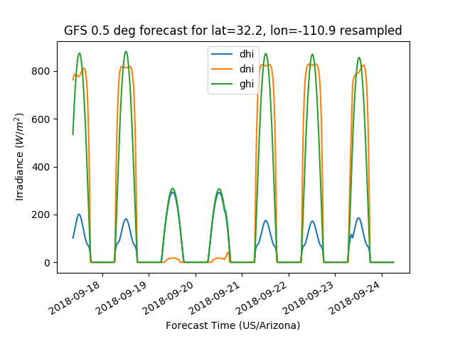
Most weather model output has a fairly coarse time resolution, at least an hour. The irradiance forecasts have the same time resolution as the weather data. However, it is straightforward to interpolate the cloud cover forecasts onto a higher resolution time domain, and then recalculate the irradiance.
In [43]: resampled_data = data.resample('5min').interpolate()

In [44]: resampled_irrads = model.cloud_cover_to_irradiance(resampled_data['total_clouds'], how='clearsky_scaling')

In [45]: resampled_irrads.plot();

In [46]: plt.ylabel('Irradiance ($W/m^2$)');

In [47]: plt.xlabel('Forecast Time ({})'.format(tz));

In [48]: plt.title('GFS 0.5 deg forecast for lat={}, lon={} resampled'
   ....:           .format(latitude, longitude));
   ....:

In [49]: plt.legend();
Users may then recombine resampled_irrads and resampled_data using
slicing pandas.concat() or pandas.DataFrame.join().
We reiterate that the open source code enables users to customize the model processing to their liking.
| [Lar16] | Larson et. al. “Day-ahead forecasting of solar power output from photovoltaic plants in the American Southwest” Renewable Energy 91, 11-20 (2016). |
| [Liu60] | B. Y. Liu and R. C. Jordan, The interrelationship and characteristic distribution of direct, diffuse, and total solar radiation, Solar Energy 4, 1 (1960). |
Weather Models
Next, we provide a brief description of the weather models available to pvlib users. Note that the figures are generated when this documentation is compiled so they will vary over time.
GFS
The Global Forecast System (GFS) is the US model that provides forecasts for the entire globe. The GFS is updated every 6 hours. The GFS is run at two resolutions, 0.25 deg and 0.5 deg, and is available with 3 hour time resolution. Forecasts from GFS model were shown above. Use the GFS, among others, if you want forecasts for 1-7 days or if you want forecasts for anywhere on Earth.
HRRR
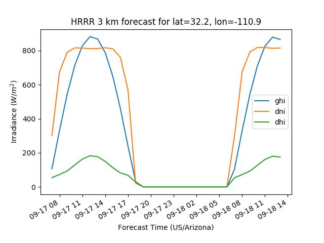
The High Resolution Rapid Refresh (HRRR) model is perhaps the most accurate model, however, it is only available for ~15 hours. It is updated every hour and runs at 3 km resolution. The HRRR excels in severe weather situations. See the NOAA ESRL HRRR page for more information. Use the HRRR, among others, if you want forecasts for less than 24 hours. The HRRR model covers the continental United States.
In [50]: model = HRRR()

In [51]: data = model.get_processed_data(latitude, longitude, start, end)

In [52]: data[irrad_vars].plot();

In [53]: plt.ylabel('Irradiance ($W/m^2$)');

In [54]: plt.xlabel('Forecast Time ({})'.format(tz));

In [55]: plt.title('HRRR 3 km forecast for lat={}, lon={}'
   ....:           .format(latitude, longitude));
   ....:

In [56]: plt.legend();
RAP
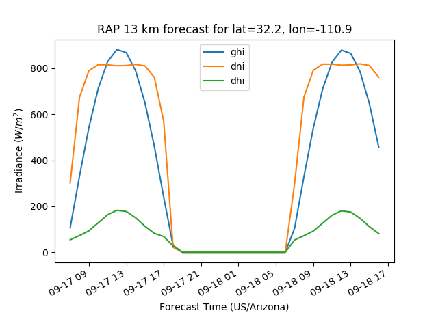
The Rapid Refresh (RAP) model is the parent model for the HRRR. It is updated every hour and runs at 40, 20, and 13 km resolutions. Only the 20 and 40 km resolutions are currently available in pvlib. It is also excels in severe weather situations. See the NOAA ESRL HRRR page for more information. Use the RAP, among others, if you want forecasts for less than 24 hours. The RAP model covers most of North America.
In [57]: model = RAP()

In [58]: data = model.get_processed_data(latitude, longitude, start, end)

In [59]: data[irrad_vars].plot();

In [60]: plt.ylabel('Irradiance ($W/m^2$)');

In [61]: plt.xlabel('Forecast Time ({})'.format(tz));

In [62]: plt.title('RAP 13 km forecast for lat={}, lon={}'
   ....:           .format(latitude, longitude));
   ....:

In [63]: plt.legend();
NAM
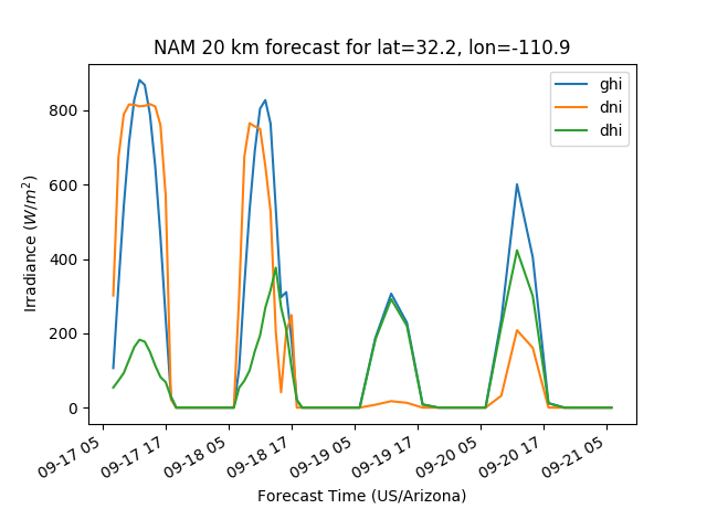
The North American Mesoscale model covers, not surprisingly, North America. It is updated every 6 hours. pvlib provides access to 20 km resolution NAM data with a time horizon of up to 4 days.
In [64]: model = NAM()

In [65]: data = model.get_processed_data(latitude, longitude, start, end)

In [66]: data[irrad_vars].plot();

In [67]: plt.ylabel('Irradiance ($W/m^2$)');

In [68]: plt.xlabel('Forecast Time ({})'.format(tz));

In [69]: plt.title('NAM 20 km forecast for lat={}, lon={}'
   ....:           .format(latitude, longitude));
   ....:

In [70]: plt.legend();
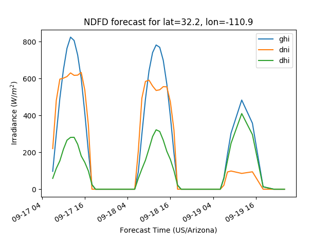
NDFD
The National Digital Forecast Database is not a model, but rather a collection of forecasts made by National Weather Service offices across the country. It is updated every 6 hours. Use the NDFD, among others, for forecasts at all time horizons. The NDFD is available for the United States.
In [71]: model = NDFD()

In [72]: data = model.get_processed_data(latitude, longitude, start, end)

In [73]: data[irrad_vars].plot();

In [74]: plt.ylabel('Irradiance ($W/m^2$)');

In [75]: plt.xlabel('Forecast Time ({})'.format(tz));

In [76]: plt.title('NDFD forecast for lat={}, lon={}'
   ....:           .format(latitude, longitude));
   ....:

In [77]: plt.legend();
PV Power Forecast
Finally, we demonstrate the application of the weather forecast data to a PV power forecast. Please see the remainder of the pvlib documentation for details.
In [78]: from pvlib.pvsystem import PVSystem, retrieve_sam

In [79]: from pvlib.tracking import SingleAxisTracker

In [80]: from pvlib.modelchain import ModelChain

In [81]: sandia_modules = retrieve_sam('sandiamod')

In [82]: cec_inverters = retrieve_sam('cecinverter')

In [83]: module = sandia_modules['Canadian_Solar_CS5P_220M___2009_']

In [84]: inverter = cec_inverters['SMA_America__SC630CP_US_315V__CEC_2012_']

# model a big tracker for more fun
In [85]: system = SingleAxisTracker(module_parameters=module,
   ....:                            inverter_parameters=inverter,
   ....:                            modules_per_string=15,
   ....:                            strings_per_inverter=300)
   ....:

# fx is a common abbreviation for forecast
In [86]: fx_model = GFS()

In [87]: fx_data = fx_model.get_processed_data(latitude, longitude, start, end)

# use a ModelChain object to calculate modeling intermediates
In [88]: mc = ModelChain(system, fx_model.location)

# extract relevant data for model chain
In [89]: mc.run_model(fx_data.index, weather=fx_data);
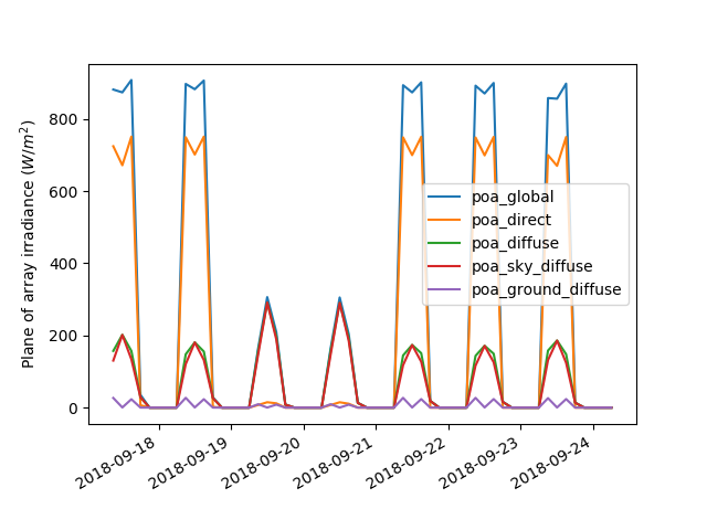
Now we plot a couple of modeling intermediates and the forecast power. Here’s the forecast plane of array irradiance…
In [90]: mc.total_irrad.plot();

In [91]: plt.ylabel('Plane of array irradiance ($W/m^2$)');

In [92]: plt.legend(loc='best');
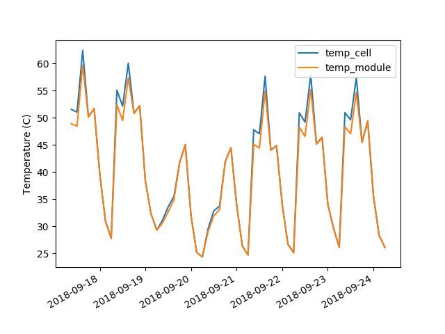
…the cell and module temperature…
In [93]: mc.temps.plot();

In [94]: plt.ylabel('Temperature (C)');
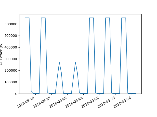
…and finally AC power…
In [95]: mc.ac.fillna(0).plot();

In [96]: plt.ylim(0, None);

In [97]: plt.ylabel('AC Power (W)');