Intro Tutorial
This page contains introductory examples of pvlib python usage.
Modeling paradigms
The backbone of pvlib-python is well-tested procedural code that implements PV system models. pvlib-python also provides a collection of classes for users that prefer object-oriented programming. These classes can help users keep track of data in a more organized way, provide some “smart” functions with more flexible inputs, and simplify the modeling process for common situations. The classes do not add any algorithms beyond what’s available in the procedural code, and most of the object methods are simple wrappers around the corresponding procedural code.
Let’s use each of these pvlib modeling paradigms to calculate the yearly energy yield for a given hardware configuration at a handful of sites listed below.
In [1]: import pandas as pd

In [2]: import matplotlib.pyplot as plt

In [3]: naive_times = pd.date_range(start='2015', end='2016', freq='1h')

# very approximate
# latitude, longitude, name, altitude, timezone
In [4]: coordinates = [(30, -110, 'Tucson', 700, 'Etc/GMT+7'),
   ...:                (35, -105, 'Albuquerque', 1500, 'Etc/GMT+7'),
   ...:                (40, -120, 'San Francisco', 10, 'Etc/GMT+8'),
   ...:                (50, 10, 'Berlin', 34, 'Etc/GMT-1')]
   ...:

In [5]: import pvlib

# get the module and inverter specifications from SAM
In [6]: sandia_modules = pvlib.pvsystem.retrieve_sam('SandiaMod')

In [7]: sapm_inverters = pvlib.pvsystem.retrieve_sam('cecinverter')

In [8]: module = sandia_modules['Canadian_Solar_CS5P_220M___2009_']

In [9]: inverter = sapm_inverters['ABB__MICRO_0_25_I_OUTD_US_208__208V_']

In [10]: temperature_model_parameters = pvlib.temperature.TEMPERATURE_MODEL_PARAMETERS['sapm']['open_rack_glass_glass']

# specify constant ambient air temp and wind for simplicity
In [11]: temp_air = 20

In [12]: wind_speed = 0
Procedural
The straightforward procedural code can be used for all modeling steps in pvlib-python.
The following code demonstrates how to use the procedural code to accomplish our system modeling goal:
In [13]: system = {'module': module, 'inverter': inverter,
....: 'surface_azimuth': 180}
....:
In [14]: energies = {}
In [15]: for latitude, longitude, name, altitude, timezone in coordinates:
....: times = naive_times.tz_localize(timezone)
....: system['surface_tilt'] = latitude
....: solpos = pvlib.solarposition.get_solarposition(times, latitude, longitude)
....: dni_extra = pvlib.irradiance.get_extra_radiation(times)
....: airmass = pvlib.atmosphere.get_relative_airmass(solpos['apparent_zenith'])
....: pressure = pvlib.atmosphere.alt2pres(altitude)
....: am_abs = pvlib.atmosphere.get_absolute_airmass(airmass, pressure)
....: tl = pvlib.clearsky.lookup_linke_turbidity(times, latitude, longitude)
....: cs = pvlib.clearsky.ineichen(solpos['apparent_zenith'], am_abs, tl,
....: dni_extra=dni_extra, altitude=altitude)
....: aoi = pvlib.irradiance.aoi(system['surface_tilt'], system['surface_azimuth'],
....: solpos['apparent_zenith'], solpos['azimuth'])
....: total_irrad = pvlib.irradiance.get_total_irradiance(system['surface_tilt'],
....: system['surface_azimuth'],
....: solpos['apparent_zenith'],
....: solpos['azimuth'],
....: cs['dni'], cs['ghi'], cs['dhi'],
....: dni_extra=dni_extra,
....: model='haydavies')
....: tcell = pvlib.temperature.sapm_cell(total_irrad['poa_global'],
....: temp_air, wind_speed,
....: **temperature_model_parameters)
....: effective_irradiance = pvlib.pvsystem.sapm_effective_irradiance(
....: total_irrad['poa_direct'], total_irrad['poa_diffuse'],
....: am_abs, aoi, module)
....: dc = pvlib.pvsystem.sapm(effective_irradiance, tcell, module)
....: ac = pvlib.pvsystem.snlinverter(dc['v_mp'], dc['p_mp'], inverter)
....: annual_energy = ac.sum()
....: energies[name] = annual_energy
....:
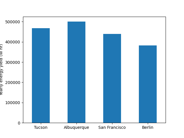
In [16]: energies = pd.Series(energies)
# based on the parameters specified above, these are in W*hrs
In [17]: print(energies.round(0))
Tucson 467494.0
Albuquerque 500230.0
San Francisco 439787.0
Berlin 383203.0
dtype: float64
In [18]: energies.plot(kind='bar', rot=0)
Out[18]: <matplotlib.axes._subplots.AxesSubplot at 0x7f51fa7d4cc0>
In [19]: plt.ylabel('Yearly energy yield (W hr)')
Out[19]: Text(0, 0.5, 'Yearly energy yield (W hr)')

Object oriented (Location, PVSystem, ModelChain)
The first object oriented paradigm uses a model where a
PVSystem object represents an assembled
collection of modules, inverters, etc., a
Location object represents a particular
place on the planet, and a ModelChain
object describes the modeling chain used to calculate PV output at that
Location. This can be a useful paradigm if you prefer to think about the
PV system and its location as separate concepts or if you develop your
own ModelChain subclasses. It can also be helpful if you make extensive
use of Location-specific methods for other calculations. pvlib-python
also includes a SingleAxisTracker class that
is a subclass of PVSystem.
The following code demonstrates how to use
Location,
PVSystem, and
ModelChain objects to accomplish our
system modeling goal. ModelChain objects provide convenience methods
that can provide default selections for models and can also fill
necessary input with modeled data. For example, no air temperature
or wind speed data is provided in the input weather DataFrame,
so the ModelChain object defaults to 20 C and 0 m/s. Also, no irradiance
transposition model is specified (keyword argument transposition for
ModelChain) so the ModelChain defaults to the haydavies model. In this
example, ModelChain infers the DC power model from the module provided
by examining the parameters defined for the module.
In [20]: from pvlib.pvsystem import PVSystem
In [21]: from pvlib.location import Location
In [22]: from pvlib.modelchain import ModelChain
In [23]: system = PVSystem(module_parameters=module,
....: inverter_parameters=inverter,
....: temperature_model_parameters=temperature_model_parameters)
....:
In [24]: energies = {}
In [25]: for latitude, longitude, name, altitude, timezone in coordinates:
....: times = naive_times.tz_localize(timezone)
....: location = Location(latitude, longitude, name=name, altitude=altitude,
....: tz=timezone)
....: weather = location.get_clearsky(times)
....: mc = ModelChain(system, location,
....: orientation_strategy='south_at_latitude_tilt')
....: mc.run_model(weather)
....: annual_energy = mc.ac.sum()
....: energies[name] = annual_energy
....:
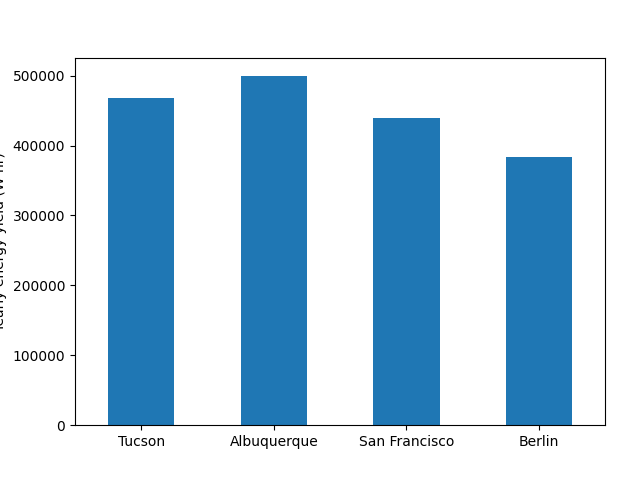
In [26]: energies = pd.Series(energies)
# based on the parameters specified above, these are in W*hrs
In [27]: print(energies.round(0))
Tucson 467459.0
Albuquerque 500151.0
San Francisco 439786.0
Berlin 383200.0
dtype: float64
In [28]: energies.plot(kind='bar', rot=0)
Out[28]: <matplotlib.axes._subplots.AxesSubplot at 0x7f51fadebd68>
In [29]: plt.ylabel('Yearly energy yield (W hr)')
Out[29]: Text(0, 0.5, 'Yearly energy yield (W hr)')
Object oriented (LocalizedPVSystem)
The second object oriented paradigm uses a model where a
LocalizedPVSystem represents a PV system at
a particular place on the planet. This can be a useful paradigm if
you’re thinking about a power plant that already exists.
The LocalizedPVSystem inherits from both
PVSystem and
Location, while the
LocalizedSingleAxisTracker inherits from
SingleAxisTracker (itself a subclass of
PVSystem) and
Location. The
LocalizedPVSystem and
LocalizedSingleAxisTracker classes may
contain bugs due to the relative difficulty of implementing multiple
inheritance. The LocalizedPVSystem and
LocalizedSingleAxisTracker may be deprecated
in a future release. We recommend that most modeling workflows implement
Location,
PVSystem, and
ModelChain.
The following code demonstrates how to use a
LocalizedPVSystem object to accomplish our
modeling goal:
In [30]: from pvlib.pvsystem import LocalizedPVSystem

In [31]: energies = {}

In [32]: for latitude, longitude, name, altitude, timezone in coordinates:
   ....:     localized_system = LocalizedPVSystem(module_parameters=module,
   ....:                                          inverter_parameters=inverter,
   ....:                                          temperature_model_parameters=temperature_model_parameters,
   ....:                                          surface_tilt=latitude,
   ....:                                          surface_azimuth=180,
   ....:                                          latitude=latitude,
   ....:                                          longitude=longitude,
   ....:                                          name=name,
   ....:                                          altitude=altitude,
   ....:                                          tz=timezone)
   ....:     times = naive_times.tz_localize(timezone)
   ....:     clearsky = localized_system.get_clearsky(times)
   ....:     solar_position = localized_system.get_solarposition(times)
   ....:     total_irrad = localized_system.get_irradiance(solar_position['apparent_zenith'],
   ....:                                                   solar_position['azimuth'],
   ....:                                                   clearsky['dni'],
   ....:                                                   clearsky['ghi'],
   ....:                                                   clearsky['dhi'])
   ....:     tcell = localized_system.sapm_celltemp(total_irrad['poa_global'],
   ....:                                            temp_air, wind_speed)
   ....:     aoi = localized_system.get_aoi(solar_position['apparent_zenith'],
   ....:                                    solar_position['azimuth'])
   ....:     airmass = localized_system.get_airmass(solar_position=solar_position)
   ....:     effective_irradiance = localized_system.sapm_effective_irradiance(
   ....:         total_irrad['poa_direct'], total_irrad['poa_diffuse'],
   ....:         airmass['airmass_absolute'], aoi)
   ....:     dc = localized_system.sapm(effective_irradiance, tcell)
   ....:     ac = localized_system.snlinverter(dc['v_mp'], dc['p_mp'])
   ....:     annual_energy = ac.sum()
   ....:     energies[name] = annual_energy
   ....:

In [33]: energies = pd.Series(energies)

# based on the parameters specified above, these are in W*hrs
In [34]: print(energies.round(0))
Tucson           467459.0
Albuquerque      500151.0
San Francisco    439786.0
Berlin           383200.0
dtype: float64

In [35]: energies.plot(kind='bar', rot=0)
Out[35]: <matplotlib.axes._subplots.AxesSubplot at 0x7f51fb0872b0>

In [36]: plt.ylabel('Yearly energy yield (W hr)')
Out[36]: Text(0, 0.5, 'Yearly energy yield (W hr)')