Fast simulation using the ADR efficiency model starting from PVsyst parameters#

Would you like to increase simulation speed by a factor of 4000+?

Simulation using single-diode models can be slow because the maximum power point is usually found by an iterative search. In this example we use the PVsyst single diode model to generate a matrix of efficiency values, then determine the ADR model parameters to approximate the behavior of the PVsyst model. This way both PVsyst and ADR models can simulate the same PV module type.

To compare simulation speed, we run them using timeit.

Author: Anton Driesse

import numpy as np
import matplotlib.pyplot as plt

from pvlib.pvsystem import calcparams_pvsyst, max_power_point
from pvlib.pvarray import fit_pvefficiency_adr, pvefficiency_adr

from timeit import timeit

Generate a matrix of power values

pvsyst_params = {'alpha_sc': 0.0015,
                 'gamma_ref': 1.20585,
                 'mu_gamma': -9.41066e-05,
                 'I_L_ref': 5.9301,
                 'I_o_ref': 2.9691e-10,
                 'R_sh_ref': 1144,
                 'R_sh_0': 3850,
                 'R_s': 0.6,
                 'cells_in_series': 96,
                 'R_sh_exp': 5.5,
                 'EgRef': 1.12,
                 }

G_REF = 1000
T_REF = 25

params_stc = calcparams_pvsyst(G_REF, T_REF, **pvsyst_params)
mpp_stc = max_power_point(*params_stc)

P_REF = mpp_stc['p_mp']

g, t = np.meshgrid(np.linspace(100, 1100, 11),
                   np.linspace(0, 75, 4))

adjusted_params = calcparams_pvsyst(g, t, **pvsyst_params)
mpp = max_power_point(*adjusted_params)
p_mp = mpp['p_mp']

print('irradiance')
print(g[:1].round(0))

print('maximum power')
print(p_mp.round(1))

irradiance
[[ 100.  200.  300.  400.  500.  600.  700.  800.  900. 1000. 1100.]]
maximum power
[[ 32.1  66.8 101.9 137.2 172.7 208.2 243.6 278.9 314.  349.  383.8]
 [ 29.6  61.7  94.4 127.4 160.5 193.6 226.7 259.7 292.5 325.2 357.7]
 [ 27.   56.6  86.9 117.4 148.1 178.8 209.5 240.2 270.7 301.  331.2]
 [ 24.4  51.4  79.2 107.2 135.5 163.8 192.1 220.4 248.5 276.5 304.4]]

Convert power matrix to efficiency and fit the ADR model to all the points

eta_rel_pvs = (p_mp / P_REF) / (g / G_REF)

adr_params = fit_pvefficiency_adr(g, t, eta_rel_pvs, dict_output=True)

for k, v in adr_params.items():
    print('%-5s = %8.5f' % (k, v))

k_a   =  1.00057
k_d   = -6.51928
tc_d  =  0.02119
k_rs  =  0.05792
k_rsh =  0.15151

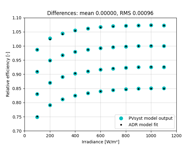
Compare the ADR model output to the PVsyst model output

eta_rel_adr = pvefficiency_adr(g, t, **adr_params)
mbe = np.mean(eta_rel_adr - eta_rel_pvs)
rmse = np.sqrt(np.mean(np.square(eta_rel_adr - eta_rel_pvs)))

plt.figure()
plt.plot(g.flat, eta_rel_pvs.flat, 'oc', ms=8)
plt.plot(g.flat, eta_rel_adr.flat, '.k')
plt.grid(alpha=0.5)
plt.xlim(0, 1200)
plt.ylim(0.7, 1.1)

plt.xlabel('Irradiance [W/m²]')
plt.ylabel('Relative efficiency [-]')
plt.legend(['PVsyst model output', 'ADR model fit'], loc='lower right')
plt.title('Differences: mean %.5f, RMS %.5f' % (mbe, rmse))
plt.show()

Generate some random irradiance and temperature data

g = np.random.uniform(0, 1200, 8760)
t = np.random.uniform(20,  80, 8760)


def run_adr():
    eta_rel = pvefficiency_adr(g, t, **adr_params)
    p_adr = P_REF * eta_rel * (g / G_REF)
    return p_adr


def run_pvsyst():
    adjusted_params = calcparams_pvsyst(g, t, **pvsyst_params)
    mpp = max_power_point(*adjusted_params)
    p_pvs = mpp['p_mp']
    return p_pvs


elapsed_adr = timeit('run_adr()', number=1, globals=globals())
elapsed_pvs = timeit('run_pvsyst()', number=1, globals=globals())

print('Elapsed time for the PVsyst model: %9.6f s' % elapsed_pvs)
print('Elapsed time for the ADR    model: %9.6f s' % elapsed_adr)
print('ADR acceleration ratio:           %9.0f x' % (elapsed_pvs/elapsed_adr))

Elapsed time for the PVsyst model:  3.203304 s
Elapsed time for the ADR    model:  0.000593 s
ADR acceleration ratio:                5404 x

That’s fast, but is it accurate? Run them again to compare the simulated power values

p_pvs = run_pvsyst()
p_adr = run_adr()

mbe = np.mean(p_adr - p_pvs)
rmse = np.sqrt(np.mean(np.square(p_adr - p_pvs)))

# sphinx_gallery_thumbnail_number = 2
plt.figure()
pc = plt.scatter(p_pvs, p_adr-p_pvs, c=t, cmap='jet')
plt.colorbar()
pc.set_alpha(0.25)
plt.ylim(-1.4, 1.4)
plt.grid(alpha=0.5)

plt.xlabel('Power calculated using the PVsyst model [W]')
plt.ylabel('ADR model power - PVsyst model power [W]')
plt.title('Differences: mean %.2f W, RMS %.2f W' % (mbe, rmse))
plt.show()

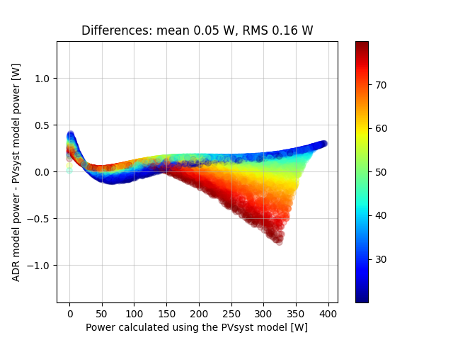
There are some small systematic differences between the original PVsyst model output and the ADR fit. But these differences are much smaller than the typical uncertainty in measured output of modules of this type. The PVsyst model and the parameters we started with are of course also only approximations of the true module behavior.

References#

1: A. Driesse and J. S. Stein, “From IEC 61853 power measurements to PV system simulations”, Sandia Report No. SAND2020-3877, 2020. DOI: 10.2172/1615179
2: A. Driesse, M. Theristis and J. S. Stein, “A New Photovoltaic Module Efficiency Model for Energy Prediction and Rating,” in IEEE Journal of Photovoltaics, vol. 11, no. 2, pp. 527-534, March 2021. DOI: 10.1109/JPHOTOV.2020.3045677

Total running time of the script: (0 minutes 6.933 seconds)

Gallery generated by Sphinx-Gallery

Simulating PV system DC output using the ADR module efficiency model

Bifacial Modeling