IAM Model Conversion

Illustrates how to convert from one IAM model to a different model using convert().

An incidence angle modifier (IAM) model quantifies the fraction of direct irradiance that is reflected away from a module’s surface. Three popular IAM models are Martin-Ruiz martin_ruiz(), physical physical(), and ASHRAE ashrae(). Each model requires one or more parameters.

Here, we show how to use convert() to estimate parameters for a desired target IAM model from a source IAM model. Model conversion uses a weight function that can assign more influence to some AOI values than others. We illustrate how to provide a custom weight function to convert().

import numpy as np
import matplotlib.pyplot as plt

from pvlib.tools import cosd
from pvlib.iam import (ashrae, martin_ruiz, physical, convert)

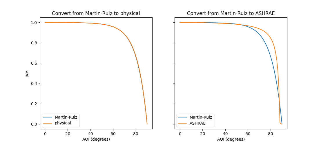
Converting from one IAM model to another model

Here we’ll show how to convert from the Martin-Ruiz model to the physical and the ASHRAE models.

# Compute IAM values using the martin_ruiz model.
aoi = np.linspace(0, 90, 100)
martin_ruiz_params = {'a_r': 0.16}
martin_ruiz_iam = martin_ruiz(aoi, **martin_ruiz_params)

# Get parameters for the physical model and compute IAM using these parameters.
physical_params = convert('martin_ruiz', martin_ruiz_params, 'physical')
physical_iam = physical(aoi, **physical_params)

# Get parameters for the ASHRAE model and compute IAM using these parameters.
ashrae_params = convert('martin_ruiz', martin_ruiz_params, 'ashrae')
ashrae_iam = ashrae(aoi, **ashrae_params)

fig, (ax1, ax2) = plt.subplots(1, 2, figsize=(11, 5), sharey=True)

# Plot each model's IAM vs. angle-of-incidence (AOI).
ax1.plot(aoi, martin_ruiz_iam, label='Martin-Ruiz')
ax1.plot(aoi, physical_iam, label='physical')
ax1.set_xlabel('AOI (degrees)')
ax1.set_title('Convert from Martin-Ruiz to physical')
ax1.legend()

ax2.plot(aoi, martin_ruiz_iam, label='Martin-Ruiz')
ax2.plot(aoi, ashrae_iam, label='ASHRAE')
ax2.set_xlabel('AOI (degrees)')
ax2.set_title('Convert from Martin-Ruiz to ASHRAE')
ax2.legend()

ax1.set_ylabel('IAM')
plt.show()

The weight function

pvlib.iam.convert() uses a weight function when computing residuals between the two models. The default weight function is \(1 - \sin(aoi)\). We can instead pass a custom weight function to pvlib.iam.convert().

In some cases, the choice of weight function has a minimal effect on the returned model parameters. This is especially true when converting between the Martin-Ruiz and physical models, because the curves described by these models can match quite closely. However, when conversion involves the ASHRAE model, the choice of weight function can have a meaningful effect on the returned parameters for the target model.

Here we’ll show examples of both of these cases, starting with an example where the choice of weight function does not have much impact. In doing so, we’ll show how to pass in a custom weight function of our choice.

# Compute IAM using the Martin-Ruiz model.
aoi = np.linspace(0, 90, 100)
martin_ruiz_params = {'a_r': 0.16}
martin_ruiz_iam = martin_ruiz(aoi, **martin_ruiz_params)

# Get parameters for the physical model ...

# ... using the default weight function.
physical_params_default = convert('martin_ruiz', martin_ruiz_params,
                                  'physical')
physical_iam_default = physical(aoi, **physical_params_default)


# ... using a custom weight function. The weight function must take ``aoi``
# as its argument and return a vector of the same length as ``aoi``.
def weight_function(aoi):
    return cosd(aoi)


physical_params_custom = convert('martin_ruiz', martin_ruiz_params, 'physical',
                                 weight=weight_function)
physical_iam_custom = physical(aoi, **physical_params_custom)

# Plot IAM vs AOI.
plt.plot(aoi, martin_ruiz_iam, label='Martin-Ruiz')
plt.plot(aoi, physical_iam_default, label='Default weight function')
plt.plot(aoi, physical_iam_custom, label='Custom weight function')
plt.xlabel('AOI (degrees)')
plt.ylabel('IAM')
plt.title('Martin-Ruiz to physical')
plt.legend()
plt.show()

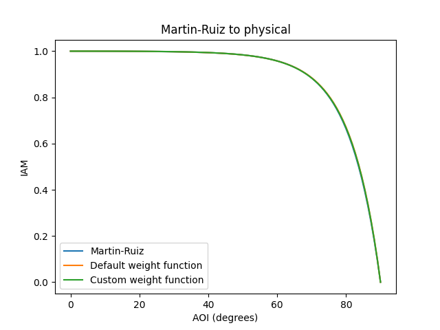
For this choice of source and target models, the weight function has little effect on the target model’s parameters.

Now we’ll look at an example where the weight function does affect the output.

# Get parameters for the ASHRAE model ...

# ... using the default weight function.
ashrae_params_default = convert('martin_ruiz', martin_ruiz_params, 'ashrae')
ashrae_iam_default = ashrae(aoi, **ashrae_params_default)

# ... using the custom weight function
ashrae_params_custom = convert('martin_ruiz', martin_ruiz_params, 'ashrae',
                               weight=weight_function)
ashrae_iam_custom = ashrae(aoi, **ashrae_params_custom)

# Plot IAM vs AOI.
plt.plot(aoi, martin_ruiz_iam, label='Martin-Ruiz')
plt.plot(aoi, ashrae_iam_default, label='Default weight function')
plt.plot(aoi, ashrae_iam_custom, label='Custom weight function')
plt.xlabel('AOI (degrees)')
plt.ylabel('IAM')
plt.title('Martin-Ruiz to ASHRAE')
plt.legend()
plt.show()

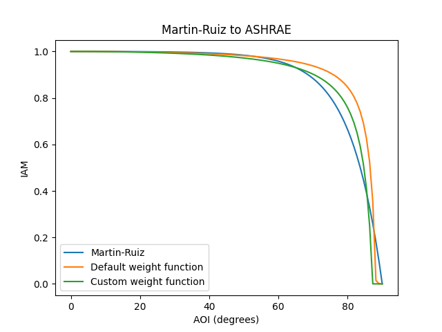
In this case, each of the two ASHRAE looks quite different. Finding the right weight function and parameters in such cases will require knowing where you want the target model to be more accurate. The default weight function was chosen because it yielded IAM models that produce similar annual insolation for a simulated PV system.

Reference

1

Jones, A. R., Hansen, C. W., Anderson, K. S. Parameter estimation for incidence angle modifier models for photovoltaic modules. Sandia report SAND2023-13944 (2023).

previous

IAM Model Fitting

next

Shading