Note
Go to the end to download the full example code.
Bifacial Modeling - procedural#
Example of bifacial modeling using pvfactors and procedural method
This example shows how to complete a bifacial modeling example using the
pvlib.pvsystem.pvwatts_dc() with the
pvlib.bifacial.pvfactors.pvfactors_timeseries() function to
transpose GHI data to both front and rear Plane of Array (POA) irradiance.
Attention
To run this example, the solarfactors package (an implementation
of the pvfactors model) must be installed. It can be installed with
either pip install solarfactors or pip install pvlib[optional],
which installs all of pvlib’s optional dependencies.
import pandas as pd
from pvlib import location
from pvlib import tracking
from pvlib.bifacial.pvfactors import pvfactors_timeseries
from pvlib import temperature
from pvlib import pvsystem
import matplotlib.pyplot as plt
import warnings

# supressing shapely warnings that occur on import of pvfactors
warnings.filterwarnings(action='ignore', module='pvfactors')

# using Greensboro, NC for this example
lat, lon = 36.084, -79.817
tz = 'Etc/GMT+5'
times = pd.date_range('2021-06-21', '2021-06-22', freq='1min', tz=tz)

# create location object and get clearsky data
site_location = location.Location(lat, lon, tz=tz, name='Greensboro, NC')
cs = site_location.get_clearsky(times)

# get solar position data
solar_position = site_location.get_solarposition(times)

# set ground coverage ratio and max_angle to
# pull orientation data for a single-axis tracker
gcr = 0.35
max_phi = 60
orientation = tracking.singleaxis(solar_position['apparent_zenith'],
                                  solar_position['azimuth'],
                                  max_angle=max_phi,
                                  backtrack=True,
                                  gcr=gcr
                                  )

# set axis_azimuth, albedo, pvrow width and height, and use
# the pvfactors engine for both front and rear-side absorbed irradiance
axis_azimuth = 180
pvrow_height = 3
pvrow_width = 4
albedo = 0.2

# explicity simulate on pvarray with 3 rows, with sensor placed in middle row
# users may select different values depending on needs
irrad = pvfactors_timeseries(solar_position['azimuth'],
                             solar_position['apparent_zenith'],
                             orientation['surface_azimuth'],
                             orientation['surface_tilt'],
                             axis_azimuth,
                             cs.index,
                             cs['dni'],
                             cs['dhi'],
                             gcr,
                             pvrow_height,
                             pvrow_width,
                             albedo,
                             n_pvrows=3,
                             index_observed_pvrow=1
                             )

# turn into pandas DataFrame
irrad = pd.concat(irrad, axis=1)

# using bifaciality factor and pvfactors results, create effective irradiance
bifaciality = 0.75
effective_irrad_bifi = irrad['total_abs_front'] + (irrad['total_abs_back']
                                                   * bifaciality)

# get cell temperature using the Faiman model
temp_cell = temperature.faiman(effective_irrad_bifi, temp_air=25,
                               wind_speed=1)

# using the pvwatts_dc model and parameters detailed above,
# set pdc0 and return DC power for both bifacial and monofacial
pdc0 = 1
gamma_pdc = -0.0043
pdc_bifi = pvsystem.pvwatts_dc(effective_irrad_bifi,
                               temp_cell,
                               pdc0,
                               gamma_pdc=gamma_pdc
                               ).fillna(0)
pdc_bifi.plot(title='Bifacial Simulation on June Solstice', ylabel='DC Power')
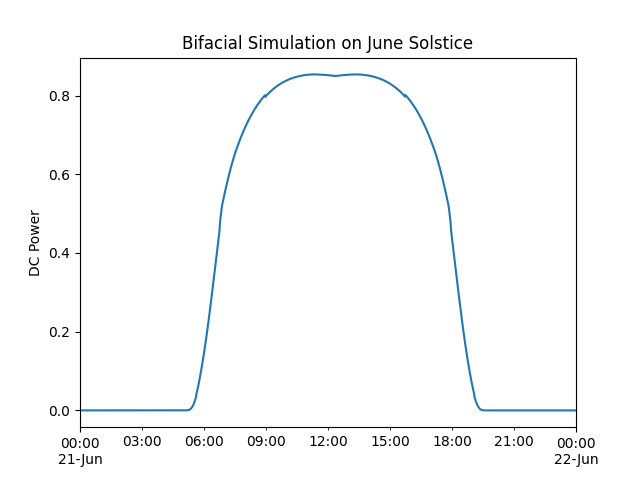
<Axes: title={'center': 'Bifacial Simulation on June Solstice'}, ylabel='DC Power'>
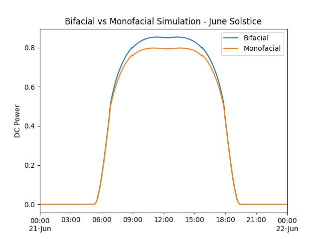
For illustration, perform monofacial simulation using pvfactors front-side irradiance (AOI-corrected), and plot along with bifacial results.
effective_irrad_mono = irrad['total_abs_front']
pdc_mono = pvsystem.pvwatts_dc(effective_irrad_mono,
                               temp_cell,
                               pdc0,
                               gamma_pdc=gamma_pdc
                               ).fillna(0)

# plot monofacial results
plt.figure()
plt.title('Bifacial vs Monofacial Simulation - June Solstice')
pdc_bifi.plot(label='Bifacial')
pdc_mono.plot(label='Monofacial')
plt.ylabel('DC Power')
plt.legend()
<matplotlib.legend.Legend object at 0x7a2ef2b883e0>
Total running time of the script: (0 minutes 0.354 seconds)