HSU Soiling Model Example

Example of soiling using the HSU model.

This example shows basic usage of pvlib’s HSU Soiling model 1 with pvlib.soiling.hsu().

References

1(1,2,3)

M. Coello and L. Boyle, “Simple Model For Predicting Time Series Soiling of Photovoltaic Panels,” in IEEE Journal of Photovoltaics. doi: 10.1109/JPHOTOV.2019.2919628

This example recreates figure 3A in 1 for the Fixed Settling Velocity case. Rainfall data comes from Imperial County, CA TMY3 file PM2.5 and PM10 data come from the EPA. First, let’s read in the weather data and run the HSU soiling model:

import pathlib
from matplotlib import pyplot as plt
from pvlib import soiling
import pvlib
import pandas as pd

# get full path to the data directory
DATA_DIR = pathlib.Path(pvlib.__file__).parent / 'data'

# read rainfall, PM2.5, and PM10 data from file
imperial_county = pd.read_csv(DATA_DIR / 'soiling_hsu_example_inputs.csv',
                              index_col=0, parse_dates=True)
rainfall = imperial_county['rain']
depo_veloc = {'2_5': 0.0009, '10': 0.004}  # default values from [1] (m/s)
rain_accum_period = pd.Timedelta('1h')     # default
cleaning_threshold = 0.5
tilt = 30
pm2_5 = imperial_county['PM2_5'].values
pm10 = imperial_county['PM10'].values
# run the hsu soiling model
soiling_ratio = soiling.hsu(rainfall, cleaning_threshold, tilt, pm2_5, pm10,
                            depo_veloc=depo_veloc,
                            rain_accum_period=rain_accum_period)

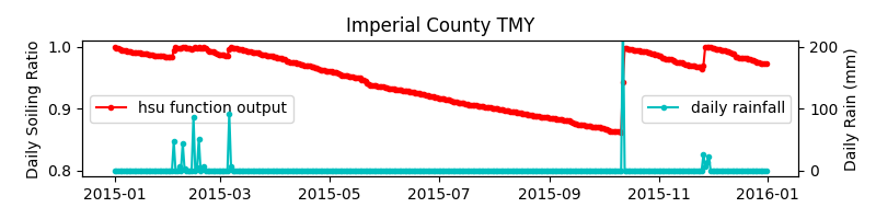
And now we’ll plot the modeled daily soiling ratios and compare with Coello and Boyle Fig 3A:

daily_soiling_ratio = soiling_ratio.resample('d').mean()
fig, ax1 = plt.subplots(figsize=(8, 2))
ax1.plot(daily_soiling_ratio.index, daily_soiling_ratio, marker='.',
         c='r', label='hsu function output')
ax1.set_ylabel('Daily Soiling Ratio')
ax1.set_ylim(0.79, 1.01)
ax1.set_title('Imperial County TMY')
ax1.legend(loc='center left')

daily_rain = rainfall.resample('d').sum()
ax2 = ax1.twinx()
ax2.plot(daily_rain.index, daily_rain, marker='.',
         c='c', label='daily rainfall')
ax2.set_ylabel('Daily Rain (mm)')
ax2.set_ylim(-10, 210)
ax2.legend(loc='center right')
fig.tight_layout()
fig.show()

Here is the original figure from 1 for comparison:

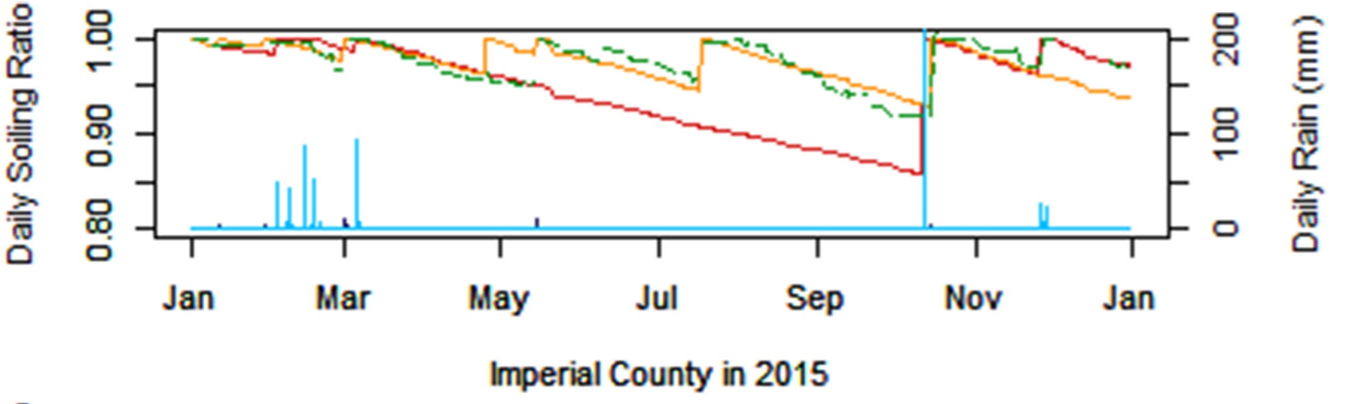
Note that this figure shows additional timeseries not calculated here: modeled soiling ratio using the 2015 PRISM rainfall dataset (orange) and measured soiling ratio (dashed green).

previous

Kimber Soiling Model

next

Solar Position