Note
Go to the end to download the full example code.
Bifacial Modeling - modelchain#
Example of bifacial modeling using pvfactors and ModelChain
This example shows how to complete a bifacial modeling example using the
pvlib.modelchain.ModelChain with the
pvlib.bifacial.pvfactors.pvfactors_timeseries() function
to transpose GHI data to both front and rear Plane of Array (POA) irradiance.
Unfortunately ModelChain does not yet support bifacial simulation
directly so we have to do the bifacial irradiance simulation ourselves.
Once the combined front + rear irradiance is known, we can pass that
to ModelChain and proceed as usual.
Future versions of pvlib may make it easier to do bifacial modeling
with ModelChain.
Attention
To run this example, the solarfactors package (an implementation
of the pvfactors model) must be installed. It can be installed with
either pip install solarfactors or pip install pvlib[optional],
which installs all of pvlib’s optional dependencies.
import pandas as pd
from pvlib import pvsystem
from pvlib import location
from pvlib import modelchain
from pvlib.temperature import TEMPERATURE_MODEL_PARAMETERS as PARAMS
from pvlib.bifacial.pvfactors import pvfactors_timeseries
import warnings

# supressing shapely warnings that occur on import of pvfactors
warnings.filterwarnings(action='ignore', module='pvfactors')

# create site location and times characteristics
lat, lon = 36.084, -79.817
tz = 'Etc/GMT+5'
times = pd.date_range('2021-06-21', '2021-6-22', freq='1min', tz=tz)

# create site system characteristics
axis_tilt = 0
axis_azimuth = 180
gcr = 0.35
max_angle = 60
pvrow_height = 3
pvrow_width = 4
albedo = 0.2
bifaciality = 0.75

# load temperature parameters and module/inverter specifications
temp_model_parameters = PARAMS['sapm']['open_rack_glass_glass']
cec_modules = pvsystem.retrieve_sam('CECMod')
cec_module = cec_modules['Trina_Solar_TSM_300DEG5C_07_II_']
cec_inverters = pvsystem.retrieve_sam('cecinverter')
cec_inverter = cec_inverters['ABB__MICRO_0_25_I_OUTD_US_208__208V_']

# create a location for site, and get solar position and clearsky data
site_location = location.Location(lat, lon, tz=tz, name='Greensboro, NC')
solar_position = site_location.get_solarposition(times)
cs = site_location.get_clearsky(times)

# load solar position and tracker orientation for use in pvsystem object
sat_mount = pvsystem.SingleAxisTrackerMount(axis_tilt=axis_tilt,
                                            axis_azimuth=axis_azimuth,
                                            max_angle=max_angle,
                                            backtrack=True,
                                            gcr=gcr)

# created for use in pvfactors timeseries
orientation = sat_mount.get_orientation(solar_position['apparent_zenith'],
                                        solar_position['azimuth'])

# get rear and front side irradiance from pvfactors transposition engine
# explicity simulate on pvarray with 3 rows, with sensor placed in middle row
# users may select different values depending on needs
irrad = pvfactors_timeseries(solar_position['azimuth'],
                             solar_position['apparent_zenith'],
                             orientation['surface_azimuth'],
                             orientation['surface_tilt'],
                             axis_azimuth,
                             times,
                             cs['dni'],
                             cs['dhi'],
                             gcr,
                             pvrow_height,
                             pvrow_width,
                             albedo,
                             n_pvrows=3,
                             index_observed_pvrow=1
                             )

# turn into pandas DataFrame
irrad = pd.concat(irrad, axis=1)

# create bifacial effective irradiance using aoi-corrected timeseries values
irrad['effective_irradiance'] = (
    irrad['total_abs_front'] + (irrad['total_abs_back'] * bifaciality)
)
With effective irradiance, we can pass data to ModelChain for bifacial simulation.
# dc arrays
array = pvsystem.Array(mount=sat_mount,
                       module_parameters=cec_module,
                       temperature_model_parameters=temp_model_parameters)

# create system object
system = pvsystem.PVSystem(arrays=[array],
                           inverter_parameters=cec_inverter)

# ModelChain requires the parameter aoi_loss to have a value. pvfactors
# applies surface reflection models in the calculation of front and back
# irradiance, so assign aoi_model='no_loss' to avoid double counting
# reflections.
mc_bifi = modelchain.ModelChain(system, site_location, aoi_model='no_loss')
mc_bifi.run_model_from_effective_irradiance(irrad)

# plot results
mc_bifi.results.ac.plot(title='Bifacial Simulation on June Solstice',
                        ylabel='AC Power')
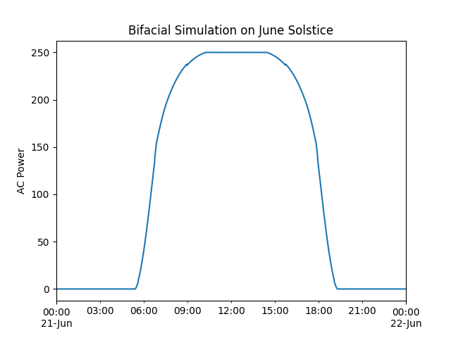
<Axes: title={'center': 'Bifacial Simulation on June Solstice'}, ylabel='AC Power'>
Total running time of the script: (0 minutes 0.455 seconds)