Note
Go to the end to download the full example code.
Diffuse Fraction Estimation#
Comparison of diffuse fraction estimation methods used to derive direct and diffuse components from measured global horizontal irradiance.
This example demonstrates how to use diffuse fraction estimation methods to obtain direct and diffuse components from measured global horizontal irradiance (GHI). Irradiance sensors such as pyranometers typically only measure GHI. pvlib provides several functions that can be used to separate GHI into the diffuse and direct components. The separate components are needed to estimate the total irradiance on a tilted surface.
import pathlib
from matplotlib import pyplot as plt
import pandas as pd
from pvlib.iotools import read_tmy3
from pvlib.solarposition import get_solarposition
from pvlib import irradiance
import pvlib

# For this example we use the Greensboro, North Carolina, TMY3 file which is
# in the pvlib data directory. TMY3 are made from the median months from years
# of data measured from 1990 to 2010. Therefore we change the timestamps to a
# common year, 1990.
DATA_DIR = pathlib.Path(pvlib.__file__).parent / 'data'
greensboro, metadata = read_tmy3(DATA_DIR / '723170TYA.CSV', coerce_year=1990,
                                 map_variables=True)

# Many of the diffuse fraction estimation methods require the "true" zenith, so
# we calculate the solar positions for the 1990 at Greensboro, NC.
# NOTE: TMY3 files timestamps indicate the end of the hour, so shift indices
# back 30-minutes to calculate solar position at center of the interval
solpos = get_solarposition(
    greensboro.index.shift(freq="-30min"), latitude=metadata['latitude'],
    longitude=metadata['longitude'], altitude=metadata['altitude'],
    pressure=greensboro.pressure*100,  # convert from millibar to Pa
    temperature=greensboro.temp_air)
solpos.index = greensboro.index  # reset index to end of the hour
pvlib Decomposition Functions#
Methods for separating GHI into diffuse and direct components include: DISC, DIRINT, Erbs, and Boland.
DISC#
DISC disc() is an empirical correlation developed
at SERI (now NLR) in 1987. The direct normal irradiance (DNI) is related to
clearness index (kt) by two polynomials split at kt = 0.6, then combined with
an exponential relation with airmass.
out_disc = irradiance.disc(
    greensboro.ghi, solpos.zenith, greensboro.index, greensboro.pressure*100)
# use "complete sum" AKA "closure" equations: DHI = GHI - DNI * cos(zenith)
df_disc = irradiance.complete_irradiance(
    solar_zenith=solpos.apparent_zenith, ghi=greensboro.ghi, dni=out_disc.dni,
    dhi=None)
out_disc = out_disc.rename(columns={'dni': 'dni_disc'})
out_disc['dhi_disc'] = df_disc.dhi
DIRINT#
DIRINT dirint() is a modification of DISC
developed by Richard Perez and Pierre Ineichen in 1992.
dni_dirint = irradiance.dirint(
    greensboro.ghi, solpos.zenith, greensboro.index, greensboro.pressure*100,
    temp_dew=greensboro.temp_dew)
# use "complete sum" AKA "closure" equation: DHI = GHI - DNI * cos(zenith)
df_dirint = irradiance.complete_irradiance(
    solar_zenith=solpos.apparent_zenith, ghi=greensboro.ghi, dni=dni_dirint,
    dhi=None)
out_dirint = pd.DataFrame(
    {'dni_dirint': dni_dirint, 'dhi_dirint': df_dirint.dhi},
    index=greensboro.index)
Erbs#
The Erbs method, erbs() developed by Daryl Gregory
Erbs at the University of Wisconsin in 1982 is a piecewise correlation that
splits kt into 3 regions: linear for kt <= 0.22, a 4th order polynomial
between 0.22 < kt <= 0.8, and a horizontal line for kt > 0.8.
out_erbs = irradiance.erbs(greensboro.ghi, solpos.zenith, greensboro.index)
out_erbs = out_erbs.rename(columns={'dni': 'dni_erbs', 'dhi': 'dhi_erbs'})
Boland#
The Boland method, boland() is a single logistic
exponential correlation that is continuously differentiable and bounded
between zero and one.
out_boland = irradiance.boland(greensboro.ghi, solpos.zenith, greensboro.index)
out_boland = out_boland.rename(
    columns={'dni': 'dni_boland', 'dhi': 'dhi_boland'})
Comparison Plots#
In the plots below we compare the four decomposition models to the TMY3 file for Greensboro, North Carolina. We also compare the clearness index, kt, with GHI normalized by a reference irradiance, E0 = 1000 [Wm⁻²], to highlight spikes caused when cosine of zenith approaches zero, particularly at sunset.
First we combine the dataframes for the decomposition models and the TMY3 file together to make plotting easier.
dni_renames = {
    'dni': 'TMY3', 'dni_disc': 'DISC', 'dni_dirint': 'DIRINT',
    'dni_erbs': 'Erbs', 'dni_boland': 'Boland'}
dni = [
    greensboro.dni, out_disc.dni_disc, out_dirint.dni_dirint,
    out_erbs.dni_erbs, out_boland.dni_boland]
dni = pd.concat(dni, axis=1).rename(columns=dni_renames)
dhi_renames = {
    'dhi': 'TMY3', 'dhi_disc': 'DISC', 'dhi_dirint': 'DIRINT',
    'dhi_erbs': 'Erbs', 'dhi_boland': 'Boland'}
dhi = [
    greensboro.dhi, out_disc.dhi_disc, out_dirint.dhi_dirint,
    out_erbs.dhi_erbs, out_boland.dhi_boland]
dhi = pd.concat(dhi, axis=1).rename(columns=dhi_renames)
ghi_kt = pd.concat([greensboro.ghi/1000.0, out_erbs.kt], axis=1)
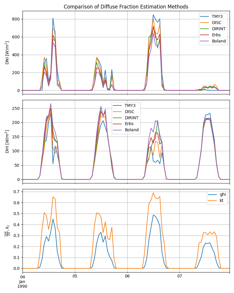
Winter#
Finally, let’s plot them for a few winter days and compare
JAN04, JAN07 = '1990-01-04 00:00:00-05:00', '1990-01-07 23:59:59-05:00'
f, ax = plt.subplots(3, 1, figsize=(8, 10), sharex=True)
dni[JAN04:JAN07].plot(ax=ax[0])
ax[0].grid(which="both")
ax[0].set_ylabel('DNI $[W/m^2]$')
ax[0].set_title('Comparison of Diffuse Fraction Estimation Methods')
dhi[JAN04:JAN07].plot(ax=ax[1])
ax[1].grid(which="both")
ax[1].set_ylabel('DHI $[W/m^2]$')
ghi_kt[JAN04:JAN07].plot(ax=ax[2])
ax[2].grid(which='both')
ax[2].set_ylabel(r'$\frac{GHI}{E0}, k_t$')
f.tight_layout()
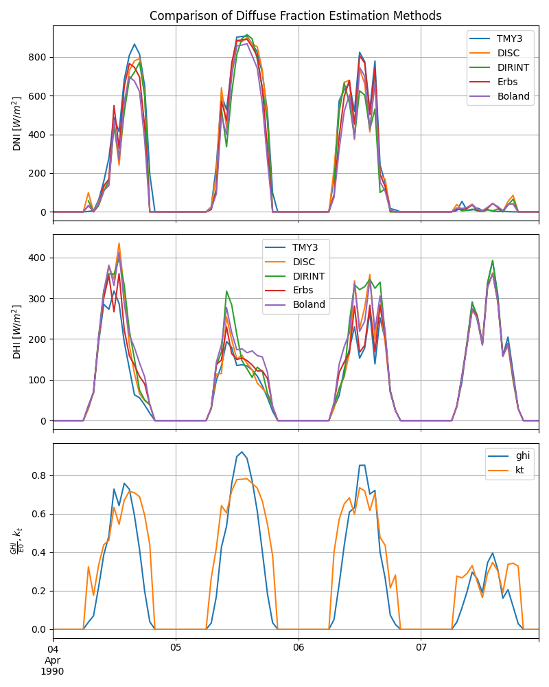
Spring#
And a few spring days …
APR04, APR07 = '1990-04-04 00:00:00-05:00', '1990-04-07 23:59:59-05:00'
f, ax = plt.subplots(3, 1, figsize=(8, 10), sharex=True)
dni[APR04:APR07].plot(ax=ax[0])
ax[0].grid(which="both")
ax[0].set_ylabel('DNI $[W/m^2]$')
ax[0].set_title('Comparison of Diffuse Fraction Estimation Methods')
dhi[APR04:APR07].plot(ax=ax[1])
ax[1].grid(which="both")
ax[1].set_ylabel('DHI $[W/m^2]$')
ghi_kt[APR04:APR07].plot(ax=ax[2])
ax[2].grid(which='both')
ax[2].set_ylabel(r'$\frac{GHI}{E0}, k_t$')
f.tight_layout()
Summer#
And few summer days to finish off the seasons.
JUL04, JUL07 = '1990-07-04 00:00:00-05:00', '1990-07-07 23:59:59-05:00'
f, ax = plt.subplots(3, 1, figsize=(8, 10), sharex=True)
dni[JUL04:JUL07].plot(ax=ax[0])
ax[0].grid(which="both")
ax[0].set_ylabel('DNI $[W/m^2]$')
ax[0].set_title('Comparison of Diffuse Fraction Estimation Methods')
dhi[JUL04:JUL07].plot(ax=ax[1])
ax[1].grid(which="both")
ax[1].set_ylabel('DHI $[W/m^2]$')
ghi_kt[JUL04:JUL07].plot(ax=ax[2])
ax[2].grid(which='both')
ax[2].set_ylabel(r'$\frac{GHI}{E0}, k_t$')
f.tight_layout()
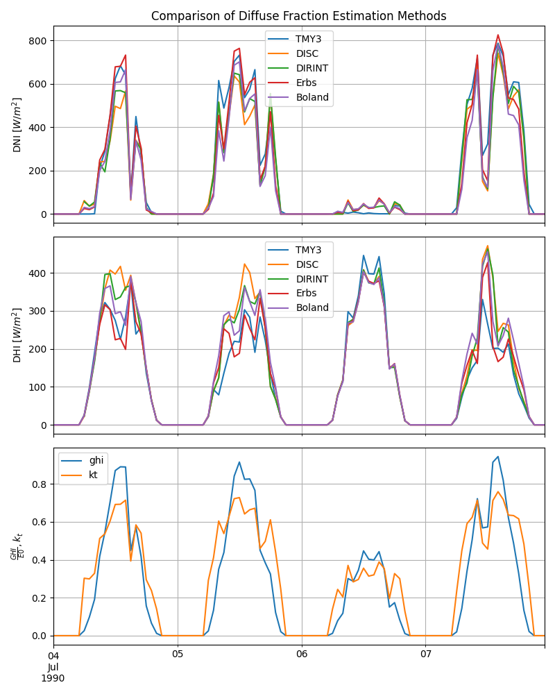
Conclusion#
This example compares several decomposition models to a TMY3 file for Greensboro, North Carolina. However, DNI and DHI in TMY3 files are themselves the output of models (either METSTAT or SUNY), and so differences between e.g. DISC output and the TMY3 file shouldn’t be regarded as errors, and it’s not a reasonable expectation to assume that the four models should reproduce the TMY3 values. We refer those interested to the TMY3 and NSRDB user manuals.
The Erbs and Boland models are correlations only based on the clearness index
kt, which is the ratio of GHI to the horizontal component of the
extra-terrestrial irradiance. At low sun elevation (zenith near 90 degrees),
especially near sunset, kt can explode because the denominator
(extra-terrestrial irradiance) approaches zero. In pvlib this behavior is
moderated by min_cos_zenith and max_clearness_index which each have
reasonable defaults. Even so, near sunset there are still spikes in kt and
DNI from Erbs and Boland for Jan. 5th & 7th, April 4th, 5th, & 7th, and July
6th & 7th.
By contrast, the DISC and DIRINT methods estimate DNI first by means of correlations, which include additional variables such as airmass. These methods seem to reduce DNI spikes over 1000 [W/m^2].
Total running time of the script: (0 minutes 1.159 seconds)