Reverse transposition limitations

Unfortunately, sometimes there is not a unique solution.

Author: Anton Driesse

Introduction

When irradiance is measured on a tilted plane, it is useful to be able to estimate the GHI that produces the POA irradiance. The estimation requires inverting a GHI-to-POA irradiance model, which involves two parts: a decomposition of GHI into direct and diffuse components, and a transposition model that calculates the direct and diffuse irradiance on the tilted plane. Recovering GHI from POA irradiance is termed “reverse transposition.”

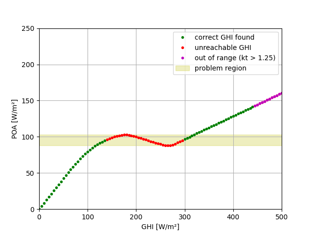
Unfortunately, for a given POA irradiance value, sometimes there is not a unique solution for GHI. Different GHI values can produce different combinations of direct and diffuse irradiance that sum to the same POA irradiance value.

In this example we look at a single point in time and consider a full range of possible GHI and POA global values as shown in figures 3 and 4 of [1]. Then we use pvlib.irradiance.ghi_from_poa_driesse_2023() to estimate the original GHI from POA global.

References

[1] (1,2,3)

Driesse, A., Jensen, A., Perez, R., 2024. A Continuous form of the Perez diffuse sky model for forward and reverse transposition. Solar Energy vol. 267. DOI: 10.1016/j.solener.2023.112093

import numpy as np

import matplotlib
import matplotlib.pyplot as plt

from pvlib.irradiance import (erbs_driesse,
                              get_total_irradiance,
                              ghi_from_poa_driesse_2023,
                              )

matplotlib.rcParams['axes.grid'] = True

Define the conditions that were used for figure 3 in [1].

dni_extra = 1366.1
albedo = 0.25
surface_tilt = 40
surface_azimuth = 180

solar_azimuth = 82
solar_zenith = 75

Define a range of possible GHI values and calculate the corresponding POA global. First estimate DNI and DHI using the Erbs-Driesse model, then transpose using the Perez-Driesse model.

ghi = np.linspace(0, 500, 100+1)

erbsout = erbs_driesse(ghi, solar_zenith, dni_extra=dni_extra)

dni = erbsout['dni']
dhi = erbsout['dhi']

irrads = get_total_irradiance(surface_tilt, surface_azimuth,
                              solar_zenith, solar_azimuth,
                              dni, ghi, dhi,
                              dni_extra,
                              model='perez-driesse')

poa_global = irrads['poa_global']

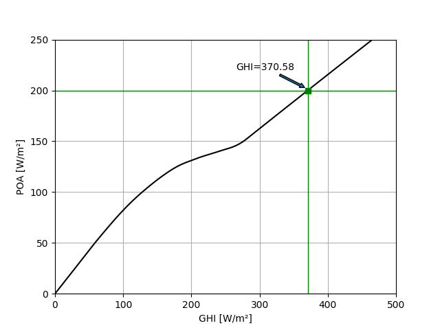
Suppose you measure that POA global is 200 W/m2. What would GHI be?

poa_test = 200

ghi_hat = ghi_from_poa_driesse_2023(surface_tilt, surface_azimuth,
                                    solar_zenith, solar_azimuth,
                                    poa_test,
                                    dni_extra,
                                    full_output=False)

print('Estimated GHI: %.2f W/m².' % ghi_hat)

Estimated GHI: 370.58 W/m².

Show this result on the graph of all possible combinations of GHI and POA.

plt.figure()
plt.plot(ghi, poa_global, 'k-')
plt.axvline(ghi_hat, color='g', lw=1)
plt.axhline(poa_test, color='g', lw=1)
plt.plot(ghi_hat, poa_test, 'gs')
plt.annotate('GHI=%.2f' % (ghi_hat),
             xy=(ghi_hat-2, 200+2),
             xytext=(ghi_hat-20, 200+20),
             ha='right',
             arrowprops={'arrowstyle': 'simple'})
plt.xlim(0, 500)
plt.ylim(0, 250)
plt.xlabel('GHI [W/m²]')
plt.ylabel('POA [W/m²]')
plt.show()

Now change the solar azimuth to match the conditions for figure 4 in [1].

solar_azimuth = 76

Again, estimate DNI and DHI using the Erbs-Driesse model, then transpose using the Perez-Driesse model.

erbsout = erbs_driesse(ghi, solar_zenith, dni_extra=dni_extra)

dni = erbsout['dni']
dhi = erbsout['dhi']

irrads = get_total_irradiance(surface_tilt, surface_azimuth,
                              solar_zenith, solar_azimuth,
                              dni, ghi, dhi,
                              dni_extra,
                              model='perez-driesse')

poa_global = irrads['poa_global']

Now reverse transpose all the POA values and observe that the original GHI cannot always be found. There is a range of POA values that maps to three possible GHI values, and there is not enough information to choose one of them. Sometimes we get lucky and the right one comes out, other times not.

result = ghi_from_poa_driesse_2023(surface_tilt, surface_azimuth,
                                   solar_zenith, solar_azimuth,
                                   poa_global,
                                   dni_extra,
                                   full_output=True,
                                   )

ghi_hat, conv, niter = result
correct = np.isclose(ghi, ghi_hat, atol=0.01)

plt.figure()
plt.plot(np.where(correct, ghi, np.nan), np.where(correct, poa_global, np.nan),
         'g.', label='correct GHI found')
plt.plot(ghi[~correct], poa_global[~correct], 'r.', label='unreachable GHI')
plt.plot(ghi[~conv], poa_global[~conv], 'm.', label='out of range (kt > 1.25)')
plt.axhspan(88, 103, color='y', alpha=0.25, label='problem region')

plt.xlim(0, 500)
plt.ylim(0, 250)
plt.xlabel('GHI [W/m²]')
plt.ylabel('POA [W/m²]')
plt.legend()
plt.show()