Note
Go to the end to download the full example code.
Modeling Spectral Irradiance#
Recreating Figure 5-1A from the SPECTRL2 NREL Technical Report.
This example shows how to model the spectral distribution of irradiance based on atmospheric conditions. The spectral distribution of irradiance is the power content at each wavelength band in the solar spectrum and is affected by various scattering and absorption mechanisms in the atmosphere. This example recreates an example figure from the SPECTRL2 NREL Technical Report [1]. The figure shows modeled spectra at hourly intervals across a single morning.
The SPECTRL2 model has several inputs; some can be calculated with pvlib, but other must come from a weather dataset. In this case, these weather parameters are example assumptions taken from the technical report.
from pvlib import spectrum, solarposition, irradiance, atmosphere
import pandas as pd
import matplotlib.pyplot as plt

# assumptions from the technical report:
lat = 37
lon = -100
tilt = 37
azimuth = 180
pressure = 101300  # sea level, roughly
water_vapor_content = 0.5  # cm
tau500 = 0.1
ozone = 0.31  # atm-cm
albedo = 0.2

times = pd.date_range('1984-03-20 06:17', freq='h', periods=6, tz='Etc/GMT+7')
solpos = solarposition.get_solarposition(times, lat, lon)
aoi = irradiance.aoi(tilt, azimuth, solpos.apparent_zenith, solpos.azimuth)

# The technical report uses the 'kasten1966' airmass model, but later
# versions of SPECTRL2 use 'kastenyoung1989'.  Here we use 'kasten1966'
# for consistency with the technical report.
relative_airmass = atmosphere.get_relative_airmass(solpos.apparent_zenith,
                                                   model='kasten1966')
With all the necessary inputs in hand we can model spectral irradiance using
pvlib.spectrum.spectrl2(). Note that because we are calculating
the spectra for more than one set of conditions, the spectral irradiance
components will be returned in a dictionary as 2-D arrays, with one dimension
for wavelength and one for time.
spectra = spectrum.spectrl2(
    apparent_zenith=solpos.apparent_zenith,
    aoi=aoi,
    surface_tilt=tilt,
    ground_albedo=albedo,
    surface_pressure=pressure,
    relative_airmass=relative_airmass,
    precipitable_water=water_vapor_content,
    ozone=ozone,
    aerosol_turbidity_500nm=tau500,
)
The poa_global array represents the total spectral irradiance on our
hypothetical solar panel. Let’s plot it against wavelength to recreate
Figure 5-1A:
plt.figure()
plt.plot(spectra['wavelength'], spectra['poa_global'])
plt.xlim(200, 2700)
plt.ylim(0, 1.8)
plt.title(r"Day 80 1984, $\tau=0.1$, Wv=0.5 cm")
plt.ylabel(r"Irradiance ($W m^{-2} nm^{-1}$)")
plt.xlabel(r"Wavelength ($nm$)")
time_labels = times.strftime("%H:%M %p")
labels = [
    "AM {:0.02f}, Z{:0.02f}, {}".format(*vals)
    for vals in zip(relative_airmass, solpos.apparent_zenith, time_labels)
]
plt.legend(labels)
plt.show()
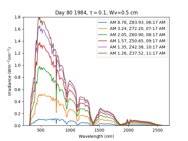
Note that the airmass and zenith values do not exactly match the values in the technical report; this is because airmass is estimated from solar position and the solar position calculation in the technical report does not exactly match the one used here. However, the differences are minor enough to not materially change the spectra.
References#
Total running time of the script: (0 minutes 0.133 seconds)